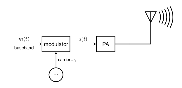
In the previous chapters we saw how to get power out of an antenna and into the air, but we conveniently ignored the question of what we actually put on the carrier. A bare sine wave at MHz carries hardly any information: it is either on or off63 . To transmit music, speech or data we have to imprint that information onto the carrier, and that imprinting is called modulation. At the receiver the reverse operation — demodulation — recovers the original signal. This chapter takes a circuits-eye view; for the communication-theory side — noise, information content, optimal detection — the standard texts of Haykin [11] and Lathi [12] are a good next step.
There are two good reasons why we do not simply connect a microphone to an antenna and transmit audio directly. Firstly, an antenna only radiates efficiently if its size is a decent fraction of the wavelength (see §11.4). At an audio frequency of kHz the wavelength is km, so a antenna would be km tall. At MHz the wavelength is m and a quarter-wave antenna is a comfortable cm. Secondly, if everybody transmitted their audio directly at baseband, all transmissions would occupy the same frequency band and interfere hopelessly. By shifting each user’s signal to a different carrier frequency we can let many transmitters share the ether without stepping on each other. Modulation solves both problems at once: it moves a low-frequency baseband signal up to a high-frequency band around a carrier.
Throughout this chapter the carrier is assumed to be a cosine
and to keep things concrete and analysable we will almost always use a single-tone modulation signal: a sine with angular frequency :
A single tone is enough to reveal the spectrum we should expect for every modulation type, and a real (audio) signal is just a sum of many such tones. In line with the philosophy of the rest of this book we will mostly assume small modulation: the carrier is only lightly perturbed by the message. This is precisely the small-signal way of thinking used for biasing amplifiers, and — as we will see — it turns the otherwise nasty non-linear modulation equations into readable, interpretable results. It is also a good description of AM broadcast (where the modulation depth is kept below ) and a reasonable first model for the frequency-modulated transmitter you will build in the project.
A useful way to sort the modulation schemes is to write the transmitted signal as a sine with a time-varying amplitude and a time-varying phase:
Everything that follows is a choice of which of these two knobs — the amplitude or the angle — carries the information:
The digital schemes ASK, PSK, FSK and QAM (§12.4) are nothing more than the same two knobs driven by a discrete levels instead of a continuous signal.
In amplitude modulation the instantaneous amplitude of the carrier is made to follow the message. Writing the amplitude as a constant plus a term proportional to ,
where the modulation index (or modulation depth)
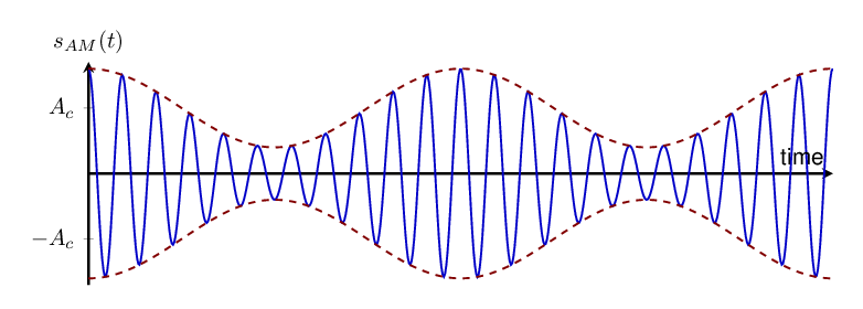
measures how deeply the carrier is modulated. For the envelope never becomes negative and the message rides on the carrier as a clean envelope, see Figure 12.2. For the envelope would try to go negative, the envelope crosses zero, and simple envelope detection at the receiver produces distortion (over-modulation). Broadcast AM is run deep — close to modulation ( up to nearly ) — to be as loud as possible, staying just below to avoid over-modulation64 . Importantly, this does not require “small” modulation: AM is linear in the message, so the three-line spectrum derived below is exact for any depth . A modest depth is needed only so that the envelope stays positive and the simple envelope detector works.
Spectrum. The product in (12.4) is turned into a sum of sines with the elementary product-to-sum identity :
So a single message tone produces exactly three lines: the carrier at and two sidebands at , each with amplitude . This is shown in Figure 12.3.
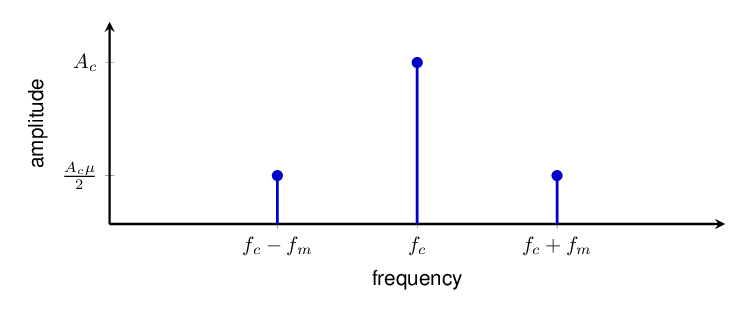
Two observations that come straight out of (12.6). First, the occupied bandwidth is : twice the highest frequency present in the message. For a kHz-limited audio signal an AM channel is therefore kHz wide. Second, the carrier itself carries no information — it is at a fixed frequency and fixed amplitude — yet in (12.6) it holds most of the power. That is wasteful, and it is why more efficient variants exist that suppress the carrier and/or one sideband (DSB-SC, SSB). Those variants save power and bandwidth but need a more elaborate receiver; classic AM keeps the carrier precisely so that the receiver can stay dead simple, as we see next.
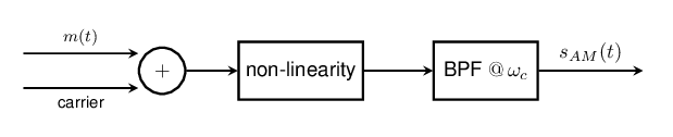
Equation (12.4) is literally a multiplication, so the most direct modulator is an analog multiplier (a mixer) that forms . In practice a full four-quadrant multiplier is not always needed; any non-linearity will do, because a non-linearity fed with the sum of the carrier and the message automatically creates the sidebands. Suppose we add carrier and message and pass them through a device with a mild square-law term — a diode or a transistor biased in a curved part of its characteristic:
The square term contains the cross-product
which is exactly the pair of sidebands, while the linear term supplies the carrier. A band-pass filter around then keeps the carrier and the two sidebands and throws away the baseband, the DC and the harmonics — and out comes an AM signal. This “sum, distort, filter” recipe is how AM was made for decades and is worth remembering: a non-linearity is a modulator.
Detection is a receiver topic, and receivers are not the focus of this book — so this and the following detection sections are background material. The whole point of keeping the carrier is that the message sits in the envelope, and an envelope is trivially cheap to recover: a diode and an RC low-pass, as in the circuit below. The diode passes only the positive peaks of the RF signal; the capacitor charges up to each peak and then holds the value, so the voltage across follows the top of the waveform — the envelope — and hence the message.
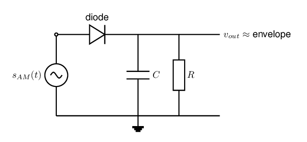
The only design rule is the choice of the time constant . It must be long compared with one carrier period so that the ripple at is smoothed away, yet short compared with one message period so that the output can still follow the fastest wiggle of the message:
This is easy exactly because ; if the envelope detector is (accidentally) dimensioned for the carrier rather than for the modulation band the detection “often goes wrong”, producing a distorted output. Note also that the diode is again a non-linearity: detection, like generation, is fundamentally a non-linear operation.
There is a catch, though, and it is not the diode’s fault. The envelope detector has no frequency selectivity of its own: it follows the envelope of whatever reaches it, the wanted station and every interferer together. It therefore has to be preceded by a band-pass filter that isolates the one wanted channel before the diode sees it. At the carrier that is a demanding filter — an AM broadcast channel is about kHz wide sitting on a carrier near MHz, so the filter must pass kHz while rejecting a neighbour only kHz away. That is a fractional bandwidth of roughly , i.e. a quality factor , and worse, it must tune to follow whichever station you select. A sharp, tunable RF filter like that is genuinely awkward to build.
There is a cleverer route that dodges the sharp filter altogether: shift the wanted band down in frequency first, and do the channel selection there. Multiplying the incoming signal by a local-oscillator sine — a mixer, the very same non-linear multiplication we used to create AM in §12.2.1 — produces sum and difference frequencies. Choosing the local oscillator near the carrier slides the wanted channel down to a low, fixed frequency (an intermediate frequency, or all the way to baseband), as in the figure below.
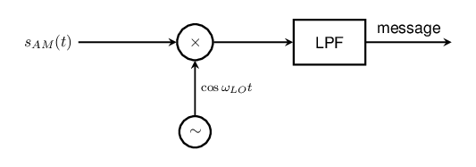
Now the channel-selecting filter is a low-pass at a low, fixed frequency, and there the same kHz is a large fractional bandwidth — a gentle, cheap, fixed filter does the job. You tune the radio by moving the local oscillator, not by re-tuning a high- filter, and whatever filtering remains at RF only has to be broad enough to knock down far-away signals and the mixing “image”, so it can be sloppy. This trade — shift the band so that the hard filtering happens at a convenient frequency — is the idea behind essentially every modern receiver [13] (the downconversion receiver, the superheterodyne, is yet another Armstrong invention, and still the dominant architecture a century later).
One refinement makes this especially clean for AM. A single mixer whose local oscillator is not phase-locked to the carrier gives an output that fades in and out as the two drift apart in phase. Using two mixers fed by local oscillators apart — an I/Q downconverter, precisely the mirror image of the I/Q modulator of §12.4 — produces an in-phase output and a quadrature output . These are the two components of the complex envelope, and the AM envelope drops straight out as
independent of the local-oscillator phase. That is exactly the diode envelope detector’s job, but done with only gentle low-pass filters and no phase lock — and, carried out with numbers instead of a diode, it is how a software-defined radio demodulates AM today.
In angle modulation the amplitude is held constant and the information is written into the argument of the cosine. This constant envelope is a real practical advantage: because the information is not in the amplitude, the transmitter’s power amplifier may clip, saturate and otherwise be driven hard and non-linearly without harming the message. That is why FM sounds clean even through a cheap, efficient, thoroughly non-linear PA65 , and it is one reason the project transmitter uses frequency modulation.
Start from the general angle-modulated signal
and define the instantaneous frequency as the time-derivative of the total argument:
The two members of the angle-modulation family differ only in what the message controls:
Phase modulation: the phase itself is proportional to the message,
Frequency modulation: the instantaneous frequency deviation is proportional to the message,
The only structural difference is an integration: FM is PM of the integral of the message, and PM is FM of the derivative of the message. If you can build one, you can build the other by adding an integrator or a differentiator in front of it.
For our single-tone message both reduce to the same shape,
with for PM and for FM, and a dimensionless modulation index . For FM,
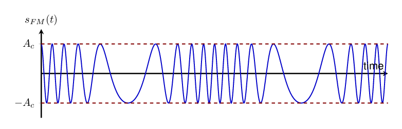
where is the peak frequency deviation: how far the instantaneous frequency swings away from at the peak of the message. For PM, is directly the peak phase deviation in radians. Figure 12.5 shows an FM waveform: the amplitude is rock-steady while the “density” of the zero crossings breathes in and out with the message.
For broadcast FM the numbers land us firmly in the wideband regime66 . With a peak deviation kHz and audio up to kHz, the modulation index is
and larger still for the lower audio tones. This is emphatically not small, so — unlike AM — we cannot linearise the cosine.
Amplitude modulation was easy because it is linear in the message: one tone gave exactly three lines. Angle modulation is non-linear — the message sits inside the cosine — and a single tone now produces a whole comb of sidebands at for . Their amplitudes turn out to be the Bessel functions of the first kind (from the Jacobi–Anger expansion; see any communications text such as [11, 12]):
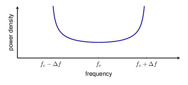
You do not need to evaluate Bessel functions by hand — the useful facts are qualitative. There are strictly infinitely many sidebands, but only about the first pairs carry appreciable power, so an FM signal behaves as if it has roughly significant sidebands spread over . Figure 12.6 shows them for : notice that the carrier line is actually quite small — most of the power has moved out into the sidebands — and that the tallest lines are the outer ones, near .
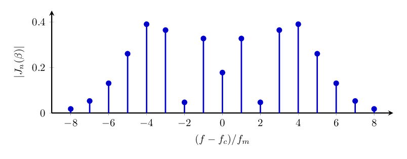
The outer lines dominate because a sinusoidally swept frequency lingers longest at the extremes of its sweep — where the instantaneous frequency turns around and — and races through the middle. The time-averaged spectrum therefore piles up at the two turning frequencies and sags in between, giving the “bathtub” envelope of Figure 12.7. That is the honest broadcast-FM spectrum for a single test tone: energy smeared across a band, not two neat sidebands.
Bandwidth. Since the sidebands reach out to about , the occupied bandwidth is no longer . A good and famous estimate is Carson’s rule [15]67 , which counts the sidebands carrying almost all the power:
For broadcast FM this gives kHz, which is why FM stations are placed on a kHz grid.
Two small ratios, one large index. It is worth separating three ratios that are easy to confuse, because for broadcast FM they are not all small:
So broadcast FM is at once a small fractional deviation of the carrier and a large modulation index, because is measured against the (small) message frequency, not against the carrier. Keeping these three apart avoids a great deal of confusion.
Excursion: narrowband FM. There is an opposite limit, , called narrowband FM. It is not the broadcast case, but it is worth a short look: it is simple, it reveals a neat duality with AM, and it has real uses — some low-data-rate two-way radios use it, and it is the first step in one classic way of building wideband FM (generate narrowband FM, then multiply the frequency up).
For we can linearise. Expanding with , and using and :
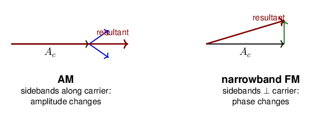
This is just the carrier plus two sidebands at , each of size — the very same three lines as AM in (12.6), with the same occupied bandwidth . The only difference from AM is a sign: the lower sideband carries a minus. That single sign is the whole difference between “the amplitude wiggles” (AM) and “the phase wiggles” (FM), and the phasor diagram of Figure 12.8 shows why. Draw the carrier as a fixed phasor and add the two sideband phasors, which counter-rotate at . In AM they add along the carrier, so the resultant grows and shrinks — amplitude modulation. The FM sign flip turns their sum perpendicular to the carrier, so the resultant tips from side to side — phase modulation — while its length barely changes.
Note there is no bathtub here: with a single sideband pair at , the energy actually sits further out than the frequency ever deviates (). The bathtub of Figure 12.7 only fills in once . The two limits are reconciled by the Bessel result (12.16): for only and survive, reproducing exactly the three lines above — sign included, since .
Making FM is refreshingly direct: we need an oscillator whose frequency depends on an input voltage, a voltage-controlled oscillator (VCO). The most general statement is that the oscillation frequency of any oscillator is fixed by its frequency-determining components,
so there is never only one component to tune and never only one way to build a VCO. The recipe is always the same: pick an element that depends on, and make that element follow the input. Which element is handiest depends on the topology — for a pure LC tank so either or will do; for a lossy resonator kept alive by an active the frequency also depends on and ; for a relaxation or – oscillator , set by a current and a capacitor.
Whatever the topology, the control handle is a non-linear component: one whose value depends on a voltage or a current across it, biased at an operating point so that a small input rides its local slope. The usual candidates are
None of this even has to be electronic. If the modulation is sufficiently slow, the tuning element can simply be moved mechanically. A mechanically variable capacitor (e.g. an air-gap (tunable) capacitor) or a variable inductor (a coil with a movable ferrite core, or a roller inductor) tunes just as well as a varicap. The prettiest example is the condenser (capacitor) microphone used as a direct modulator: the sound pressure moves one plate of a capacitor sitting in the tank, so the audio itself becomes and the oscillator is frequency-modulated with no electronics in between. Mechanical inertia sets the ceiling here — such tuning follows audio comfortably but cannot keep up with fast modulation — which is exactly why the electronic handles above take over as soon as the modulation frequency rises.
Note that a tunable component together with a fixed complementary component may behave like a tunable version of that complement. For example, a varicap in series with a fixed inductor presents a net positive reactance that varies with the control voltage — an electronically “tunable inductor” built from a fixed inductor and a varicap.
The amount of frequency deviation follows from a small-signal calculation, done in the usual small-signal way. For example, differentiating with respect to the tank capacitance,
where the modulation signal dependent converts the modulation signal into frequency shifts. Assuming 68, the peak frequency deviation for a modulation signal amplitude is
which is the modulator’s “gain” in Hz per volt. Everything you need to design the modulation depth of your transmitter is in this one line: pick the operating point on the varicap’s curve (which sets ), and know what fraction of the tank the varicap represents (which sets ). This is precisely the operating-point-plus-small-signal reasoning from the amplifier chapters, now applied in the frequency domain.
Detecting FM — again a receiver topic, and so background material — means turning the frequency variations back into a voltage. Several approaches exist, and, as with AM, all of them become easier if the signal is first mixed down to a lower fixed frequency (§12.2.3), where the same deviation is a larger fractional swing and the components are gentler [11, 12]. The bare basics are:
Digital modulation is a step beyond what the project needs — the transmitter you build is analog FM — so this whole section is background material, a short look at how the same two knobs carry bits for the reader who wants the link to modern radio. When the message is digital — a stream of bits — the amplitude and the angle are simply switched between discrete values [17]. The three elementary schemes map one-to-one onto the analog ones:
A compact way to picture and to compare these schemes is the constellation diagram shown below. Write the transmitted signal in terms of an in-phase and a quadrature component,
and plot each allowed symbol as a point . Distance from the origin is amplitude; angle is phase. Each scheme is then just a pattern of dots.
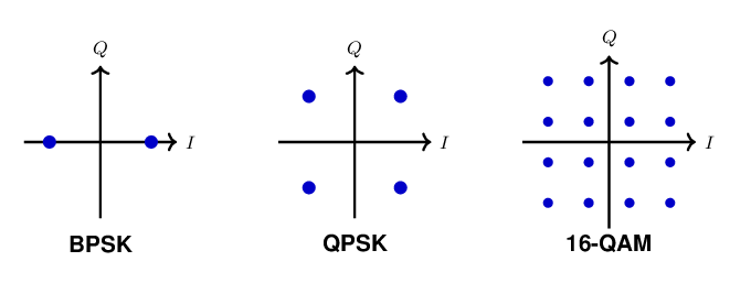
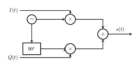
QAM (quadrature amplitude modulation) is the general case and the workhorse of modern digital links (Wi-Fi, cable, LTE). It uses both amplitude and phase: the and values are chosen independently from a grid, so a single symbol can carry many bits (16-QAM carries 4 bits, 256-QAM carries 8). The relation above also is the recipe for building it: the I/Q modulator shown below takes two baseband signals and , multiplies them by two carriers that are apart, and adds the results. Choosing and appropriately produces any of the schemes above — ASK, PSK and QAM are all just different sets of points fed into the same hardware [13]. It is a genuinely unifying picture: one modulator, many modulations.
Two general remarks close the section. First, bandwidth: an abrupt switch between symbols contains fast edges, and fast edges are wide in frequency. A keyed carrier at a symbol rate occupies a main spectral lobe of width around (the Fourier transform of a rectangular symbol is a ), with skirts that must usually be tamed by pulse-shaping filters so as not to spill into the neighbours’ channels. Second, the trade-off: packing more points into the constellation sends more bits per symbol without using more bandwidth, but the points crowd together and a given amount of noise is then more likely to push a received point into the wrong decision region. Choosing a constellation is choosing a point on the eternal engineering trade between data rate, bandwidth, power and robustness.
Figure 10.1 shows a rather simple representation of a transmit and receive system. The figure below depicts a more complete representation, where the signal to be transmitted is applied to a block that takes care of the modulation onto an RF carrier frequency. For transmitting e.g. audio in the FM band this block changes the oscillation frequency — about a center frequency — in proportion to the input signal. For audio broadcast FM this center frequency is between 88 MHz and 108 MHz while the frequency modulation is lower than 100 kHz. Note that this is a small frequency modulation on a bias frequency: very similar to the biasing and small signal operation of amplifiers.
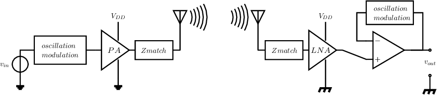
As described in§11.4, the antenna impedance can be heavily reactive (inductive or capacitive) which makes a rubbish load impedance. The (optional) “Zmatch” block between the power amplifier and the antenna ensures that the load impedance seen from the PA is optimal for the PA. This optimum impedance ideally is purely resistive with a suitable resistive value.
The receiver block looks quite a bit like the transmit part. Firstly, the antenna signal is amplified using something called a Low-Noise Amplifier to amplify the small antenna signal without adding a lot of noise. Demodulation can be done in a number of ways. In the figure, the inverse of the modulation operation is used to retrieve the original signal . Also this can be done in a number of ways; the simplest of which is using a feedback system with transfer as shown in Figure 12.9. The only difference with the systems from chapters 6 and 7 is that the opamp block for FM demodulation has its input signal in the frequency domain, with the output signal in the voltage domain. Then the “opamp” input circuit compares frequencies; using the transmitter’s modulator in the feedback loop effectively demodulates the FM-modulated input signal. The hard part is usually getting sufficient gain and sufficiently low noise at the high frequencies used. Diving into receivers is not a subject of this book.
This chapter and the earlier RF chapters converge on a small transmit system: a circuit that takes a baseband signal — audio, say — puts it on a carrier by one of the modulation schemes above, and radiates it. Nothing in what follows is tied to a particular frequency or a particular modulation. Any carrier above roughly MHz already behaves in the “RF” way this chapter assumes; the commercial FM broadcast band (–MHz) is a convenient target only because you can then pick up your own signal on any FM radio or a cheap software-defined radio, and frequency modulation is a natural choice because its constant envelope tolerates a hard-driven, efficient output stage (§12.3).
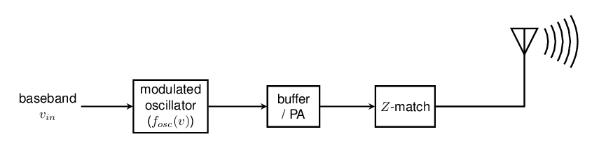
A word on why the buffer earns its place. The oscillator’s frequency is set by a lightly-loaded resonant tank, and anything that loads that tank — including a reactive, wandering antenna impedance — will pull the frequency and can even stop oscillation. Isolating the tank from the antenna with a buffer keeps the frequency stable and hands the job of delivering power to a stage that is allowed to be driven hard.
What makes such a system a fitting capstone for this book is that it draws on almost all of it at once, and the threads are worth pulling together explicitly.