Introduction to RF electronics

10 Introduction to RF electronics

10.1 Introduction

Radio frequency circuitry (RF-circuits) are different from normal (low-frequency) circuits. One hint in this direction could be the radio within the term itself. With this term, we do not only aim at an AM-radio, FM-radio or such, but at an arbitrary circuit or system that can transmit or receive RF signals. All electronic circuits which have some form of wireless communication are RF-circuits. It does not matter whether it is AM, FM, PM, Bluetooth, IEEE 802.11, GSM, 4G or something else: these are merely the protocols.

Transmitting and receiving data is something completely different from what we have covered so far. The laws of Ohm and Kirchhoff could (almost) always be applied within this book. However, these laws do not allow us to transmit data wirelessly: there is no wire between transmitter⁵⁶ and receiver, meaning that there is no current loop or voltage mesh. Hence, it would be impossible to transmit information. Compare it with cutting the cord of your iPod earplugs: the current loop is broken, hence there is no more sound⁵⁷ .

There are exceptions, for example a transformer or a capacitor. A transformer consists of two coupled inductors. One of these inductors is driven by an (AC) input signal and generates a (AC) magnetic field, while the other inductor transforms this field back into an (AC) output signal. The overall result is a fixed ratio between the current and voltage at the primary and secondary side of the transformer, without any wire between the primary and secondary side... A capacitor does not have a true electrical path between the two plates either: there is an insulating layer between the plates. In a capacitor the conduction takes place via charge storage at the plates, as a response to an electric field between the plates of the capacitor. The (AC) current through the capacitor occurs only if an AC voltage is applied.

Both effects in the transformer and in the capacitor are a lot like transmitting — transfer of electric signals without a closed conductive path — and are obviously related to actual transmitting. However, the subtle difference is that in a capacitor and in a transformer the transmitter and receiver are very closely spaced: it’s the other plate in a capacitor or the coupled inductor in a transformer. With a radio system, you are transmitting power, whether or not it is absorbed by any receiver at any distance. More on this later.

The main difference between low-frequency electronics and radio-frequency (RF) electronics is that at low frequencies the voltage law, current law and such are true while at RF the propagation speed of the signals and the theory of relativity are important⁵⁸ . This is comparable with the fact that Newtonian (mechanical) laws apply for objects at low speeds, but do not apply at very high speeds: relativity starts to come into play. You wouldn’t really notice the effects of relativity in every day mechanics, but you will in every days electronics.

10.2 Transmitting and receiving

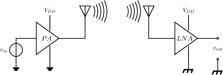
Figure 10.1 shows a basic transmitting/receiving system. At the transmitting side, the signal is amplified with a power amplifier (PA) and fed into an antenna. For simplicity reasons, let’s assume any of the widely applied antenna’s that measure $z_{𝑎𝑛𝑡𝑒𝑛𝑛𝑎} \to \infty Ω$ using a regular multimeter.

According to Kirchhoff’s voltage law, current law and Ohm’s law this should yield a zero current in the antenna as there is no closed loop at the output of the PA including the antenna. As a result the (real) power going into the antenna should be — from a low frequency point-of-view — zero. Consequently, zero (real) power would be dissipated in the antenna and hence no power would be transmitted. After reading this chapter, you’ll know better: the antenna generates an (AC) electromagnetic wave from its (AC) input voltage and thereby converts electrical energy into electromagnetic energy. In the electrical domain the antenna then presents a finite and on-zero resistance and may also include a reactive component: the antenna is a device that may store electrical energy but also converts electrical energy into energy in another domain.

pict — Figure 10.1: A transmit-receive system: a signal is transmitted wirelessly

A proper transmitting antenna — that can transmit on a specific frequency and/or in a specific direction — can also receive at the same frequency from the same direction. At the receiver side, the receiving antenna⁵⁹ transforms the electromagnetic wave back to a voltage or current, from which the original $v_{𝑖𝑛}$ can be obtained. Typically a (low noise) amplifier — represented by the LNA block — is present at the receive side to significantly amplify the (small) antenna signal.

The received power by the receive antenna is related to the transmitted power, as described by the Friis equation:

\begin{array}{rcl} P_{𝑟𝑒𝑐𝑒𝑖𝑣𝑒𝑟} & = P_{𝑡𝑟𝑎𝑛𝑠𝑚𝑖𝑡𝑡𝑒𝑟} \cdot G_{𝑡𝑟𝑎𝑛𝑠𝑚𝑖𝑡𝑡𝑒𝑟} \cdot G_{𝑟𝑒𝑐𝑒𝑖𝑣𝑒𝑟} \cdot {(\frac{λ}{4 𝜋𝑅})}^{2} \\ with & λ the wavelength of the EM-wave \\ R the distance between the transmitter and receiver antennae \end{array}

The factors $G_{𝑡𝑟𝑎𝑛𝑠𝑚𝑖𝑡𝑡𝑒𝑟}$ and $G_{𝑟𝑒𝑐𝑒𝑖𝑣𝑒𝑟}$ are the gain factors of the antenna in the direction of the other antenna. Antenna gain and antenna directivity are not covered in detail in this book: only §11.6 touches a number of antenna characteristics, including gain and directivity. For now, let’s simply assume that the antenna is not direction sensitive; then $G_{𝑟𝑒𝑐𝑒𝑖𝑣𝑒𝑟} = G_{𝑡𝑟𝑎𝑛𝑠𝑚𝑖𝑡𝑡𝑒𝑟} = 1$ . Hence, within this book, we use:

\begin{array}{rcl} P_{𝑟𝑒𝑐𝑒𝑖𝑣𝑒𝑟} & \approx & P_{𝑡𝑟𝑎𝑛𝑠𝑚𝑖𝑡𝑡𝑒𝑟} \cdot {(\frac{λ}{4 𝜋𝑅})}^{2} & (10.1) \end{array}

The above relation already shows that for large distances between transmitter and receiver — which is usually the case — the received power is quite a bit smaller than the transmitted power. In this chapter the focus is mainly on getting a high transmitting power. Since the transmitting and receiving antennae are assumed to be identical, this should also give us a high(er) receiving power. For a high transmitting power, we need:

a large output voltage from our PA.
This has already been covered in this book. For low-frequency amplifiers — up to a few MHz — we can use op-amps; for higher frequencies we need single-transistor circuits.
to get the output voltage of the PA at the feed point of the antenna.
This is fairly straightforward for low frequencies: the amplifier’s output voltage can simply be routed to the antenna. However, for RF frequencies this is a bit more complicated as explained briefly in §11.1. No in-depth analysis is given in this book.
the antenna to efficiently transform the input voltage at the feed point into transmitted power. After a brief introduction to antennae in §11.3, we will discuss the dipole antenna in §11.4 and monopole antenna in §11.5. Other types of antennae are not covered in this book.

An RF-system usually transmits a (modulated) sine wave. As you will see further on in this chapter, the antenna can — from an electronics point-of-view — be modelled as an impedance $Z_{𝑎𝑛𝑡𝑒𝑛𝑛𝑎} = R_{𝑎𝑛𝑡𝑒𝑛𝑛𝑎} + j X_{𝑎𝑛𝑡𝑒𝑛𝑛𝑎}$ . In this, the real part $R_{𝑎𝑛𝑡𝑒𝑛𝑛𝑎}$ models the conversion of electrical energy into (here) radiated electromagnetic radiation. The imaginary part $j X_{𝑎𝑛𝑡𝑒𝑛𝑛𝑎}$ models the energy storage around the antenna which is very much the same as energy storage in capacitors and inductors. In conventional circuit theory, energy storage in an element gives rise to reactive power. From this it follows that:

\begin{array}{rcl} P_{𝑡𝑟𝑎𝑛𝑠𝑚𝑖𝑡} & \equiv P_{𝑎𝑛𝑡𝑒𝑛𝑛𝑎, 𝑟𝑒𝑎𝑙} = P_{R_{𝑎𝑛𝑡𝑒𝑛𝑛𝑎}} \\ P_{𝑟𝑒𝑎𝑐𝑡𝑖𝑣𝑒} & \equiv P_{𝑎𝑛𝑡𝑒𝑛𝑛𝑎, 𝑖𝑚𝑎𝑔} = P_{X_{𝑎𝑛𝑡𝑒𝑛𝑛𝑎}} \end{array}

Using conventional network theory, it can be derived that the transmitted power and reactive power are given by:

\begin{array}{rcl} P_{𝑡𝑟𝑎𝑛𝑠𝑚𝑖𝑡} & = & \frac{V \cdot I}{2} \cdot \cos (𝜃_{v} - 𝜃_{i}) \\ P_{𝑟𝑒𝑎𝑐𝑡𝑖𝑣𝑒} & = & \frac{V \cdot I}{2} \cdot \sin (𝜃_{v} - 𝜃_{i}) \end{array}

Where $V$ and $I$ represent the voltage and current amplitudes; the factor 2 is introduced because of the ratio between effective value and magnitude for a sinusoidal signal. It’s usually easier not to work with the relations above, but with

\begin{array}{rcl} P_{𝑡𝑟𝑎𝑛𝑠𝑚𝑖𝑡} & = & I_{𝑒𝑓𝑓}^{2} \cdot 𝑅𝑒 (Z_{𝑎𝑛𝑡𝑒𝑛𝑛𝑎}) \end{array}

where $I_{𝑒𝑓𝑓}$ can usually be found from an expression including the voltage applied to the feed point of the antennae and the total antenna-impedance. Using Ohm’s law this yields:

\begin{array}{rcl} I & = & \frac{V}{Z_{𝑎𝑛𝑡𝑒𝑛𝑛𝑎}} \\ | I | & = & \frac{| V |}{| Z_{𝑎𝑛𝑡𝑒𝑛𝑛𝑎} |} \\ . . . \end{array}

This allows for easy calculation of the (real) transmitted power, once the effective voltage (or amplitude or ...) on the feed point of the antenna is known. For example, for an voltage amplitude $V$ applied to the antenna:

\begin{array}{rcl} P_{𝑡𝑟𝑎𝑛𝑠𝑚𝑖𝑡} & = & \frac{V^{2}}{2 \cdot | Z_{𝑎𝑛𝑡𝑒𝑛𝑛𝑎} |^{2}} \cdot 𝑅𝑒 (Z_{𝑎𝑛𝑡𝑒𝑛𝑛𝑎}) \end{array}

Some basics of antennas are explained in chapter 11 whereas basics of modulation are described in chapter 12. Finally, some RF-specifics are discussed in chapter 13. Note that these are (2026) mainly important for the Electronics projects.

[prev] [prev-tail] [front] [up]