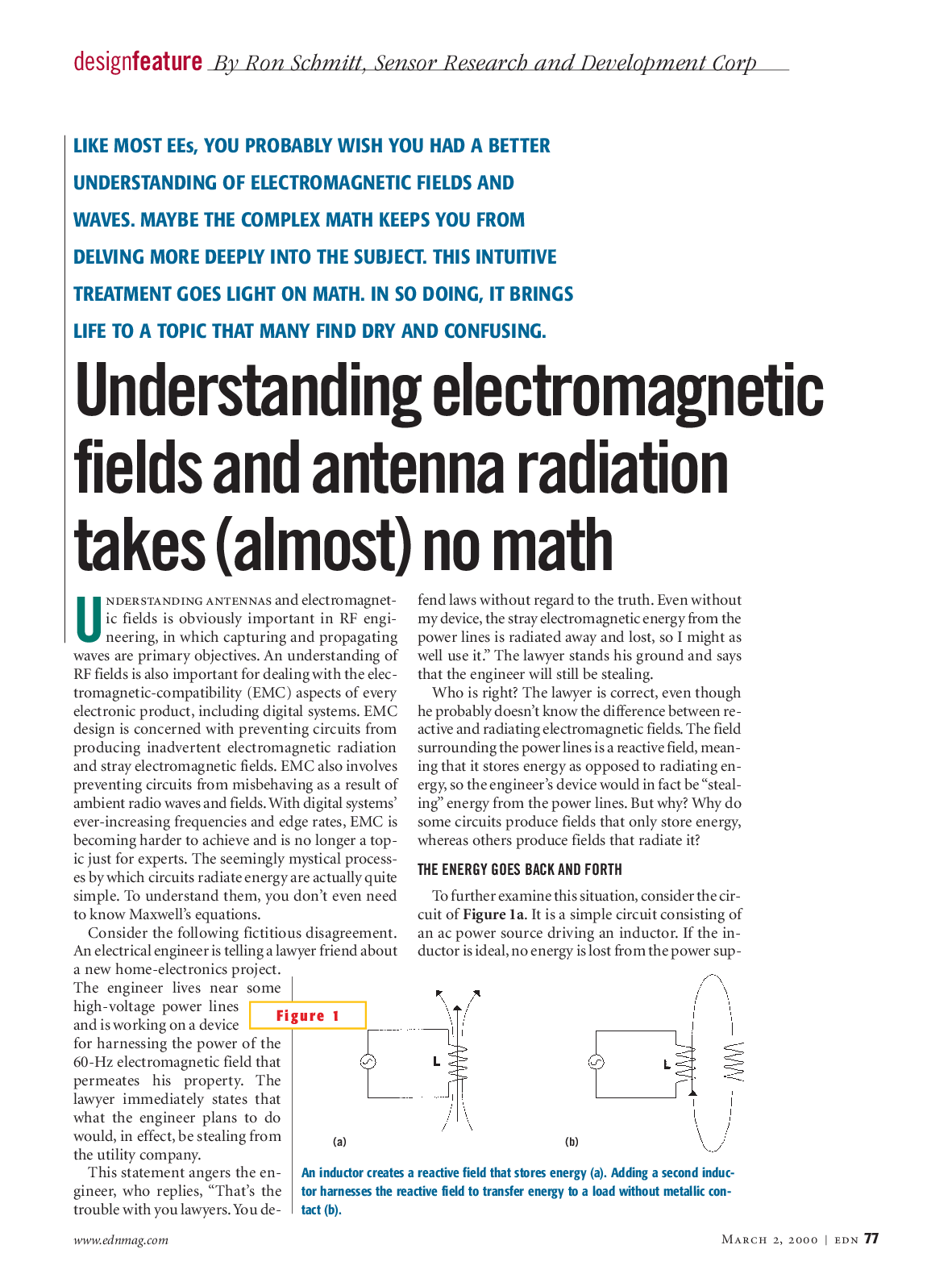
An antenna is the component that turns the transmitter’s electrical signal into a radiated electromagnetic wave — and, at the receiver, turns the wave back into a signal. This chapter first recaps the Maxwell background that explains why a structure radiates and when Kirchhoff’s laws stop applying, and then treats the dipole and monopole antenna as circuit elements: impedances that you can actually design and calculate with.
The laws of Maxwell relate the electric field to charge, current and the magnetic field:
Here, is the electric field, the magnetic field and and are the well known operators for vector calculus: the rotation and divergence. As the names of these operations already suggest, these operators calculate how much a vector field rotates or changes. We will not go into these operations and equations: we will work towards a — within the context of this book — usable result. The magnetic field is related to currents and voltages through relativity, meaning that the constants and are related to the speed of light :
It follows from (11.1) that a change in -field causes a change in -field, and vice versa. From the vector operations, it also follows that the -field caused by a time-varying -field is perpendicular to that -field. The same holds for an -field caused by a time-varying -field: this is also perpendicular to . It now can be derived that the power density of the and fields (called an EM-field) is given by the so-called Poynting vector, which is perpendicular to the and fields60:
| (11.2) |
The Maxwell equations are an expansion of the voltage and current laws of Kirchhoff. This can also be seen from the equations themselves: for any mesh using the voltage law:
For the same mesh, a similar equation can be written down in terms of electric field strength . The summation then becomes a contour integral — an integral over a closed contour — and results in:
The integral form of is given by . Here, is the total magnetic flux through the surface that is enclosed by the contour. Trying to equate the Maxwell relation equal to the Kirchhoff voltage law relation reveals that:
We can derive something similar for Kirchhoff’s current law. If we take the divergence of Ampère’s law — the Maxwell equation for — then we get61for any 3-dimensional vector:
This relation states that the change in current (density) in a certain volume is due to the accumulation of charge within that volume. This accumulation happens for every current or voltage change, since charge cannot leave infinitely fast from that volume.Trying to equate the KCL to the Maxwell result above, it follows that:
In all previous chapters in this book, the analyses were based on Kirchhoff’s voltage and current law. This implicitly means that the signal frequencies must be low enough: low enough for the wavelength of an EM-wave to be much larger than the physical dimensions of the circuit. For an audio amplifier, which has to operate up to 20 kHz, these assumptions are true if the amplifier is much smaller than 15 km, which is usually satisfied. For a GSM in the 1.8 GHz band however, this already becomes a problem. In this case, the entire circuit must be much smaller than 15 cm to be able to use the current and voltage laws. The internal IC’s within the GSM typically are much smaller than this 15cm and then can be designed and analyzed using the KVL and KCL, but as soon as you connect these ICs with something at the outside — a package, matching network or antenna — then the distances increase to such an extent that the laws of Kirchhoff are not applicable anymore.
A basic rule? Well alright: in general, you may use the Kirchhoff laws if the dimensions of the circuit are smaller than .
An antenna is driven at its feed point by a voltage and transmits an electromagnetic (EM) wave; this course does not analyze the physics behind antennae in detail. From a circuit or system perspective it is only important that the antenna does transmit or receive, and that you can model the antenna behavior by an impedance .
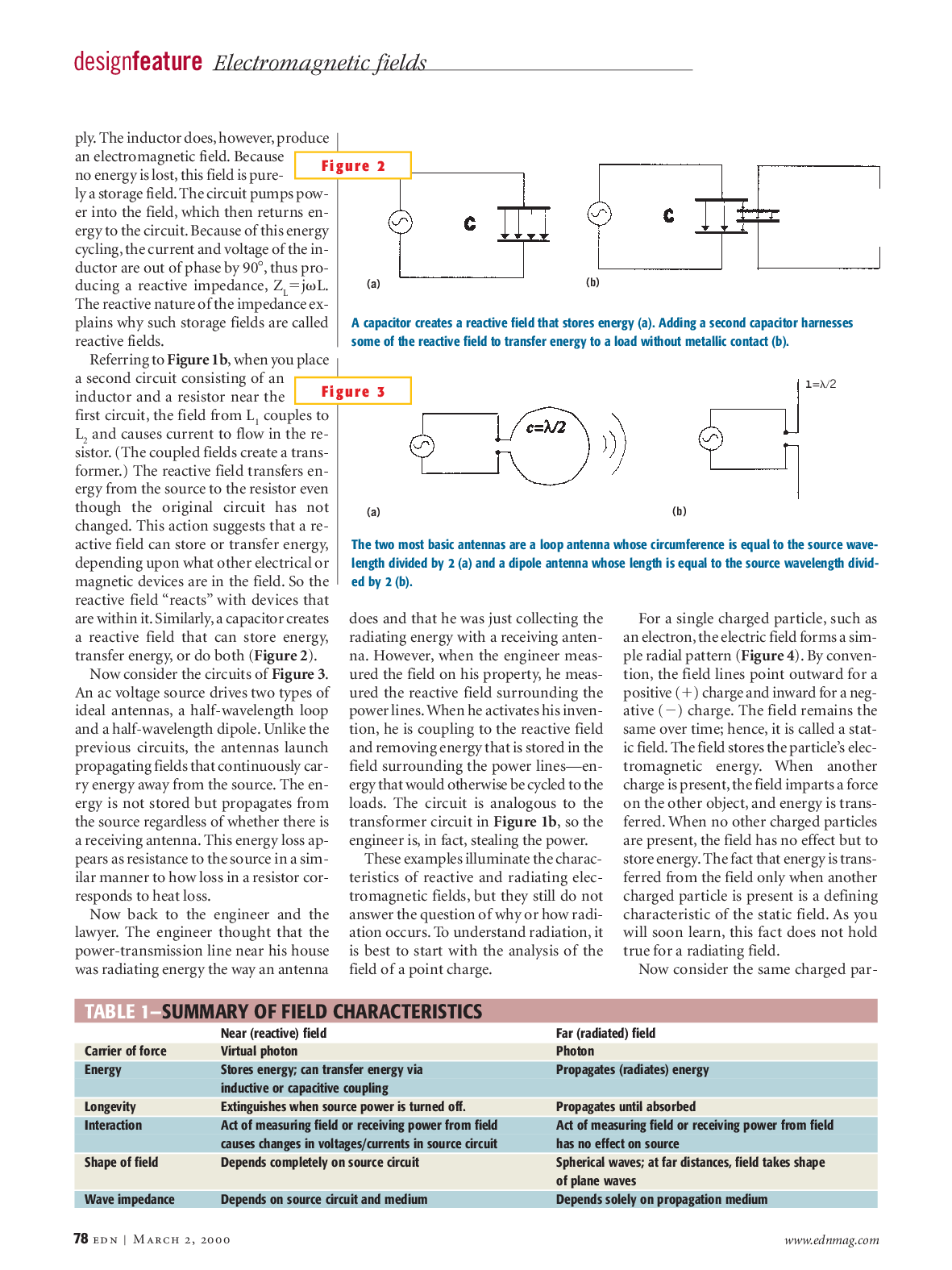
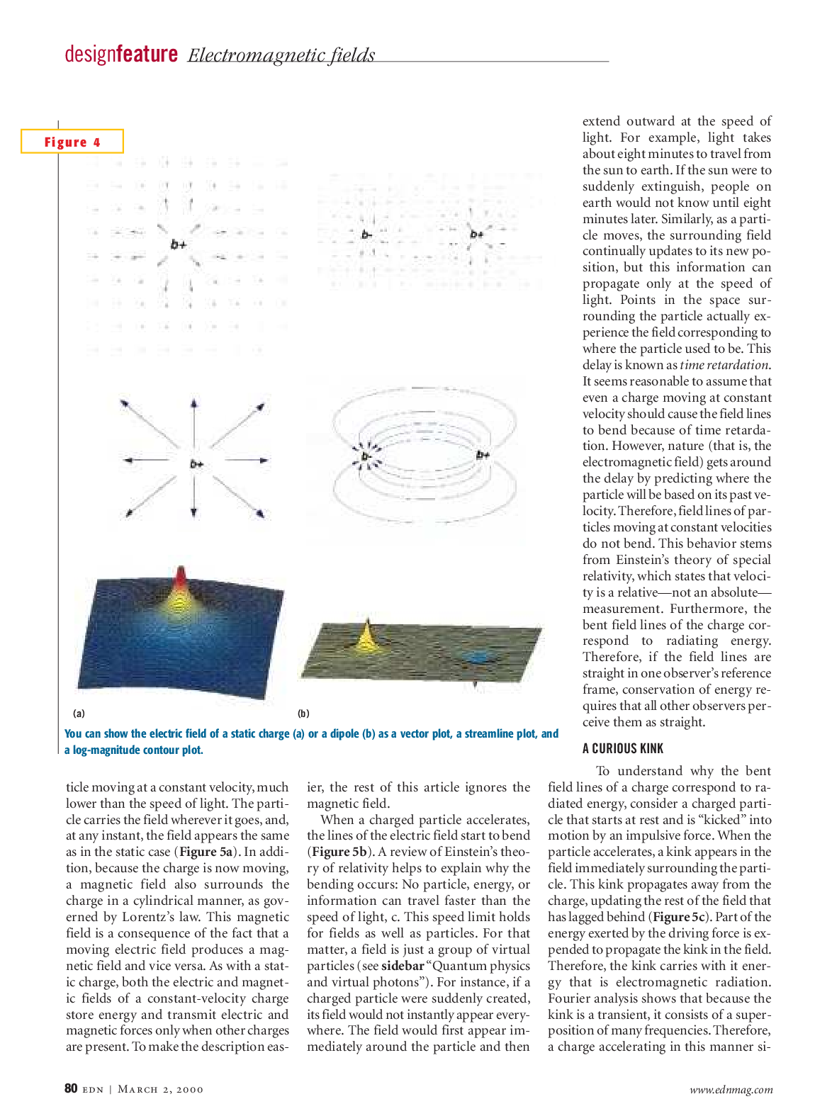
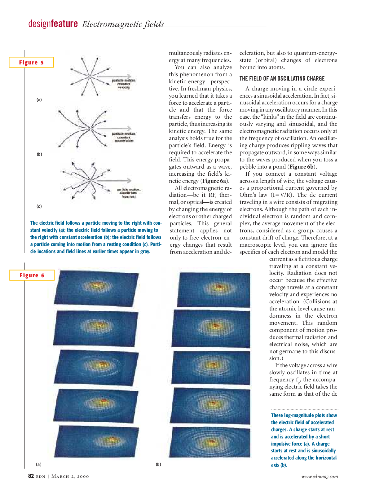
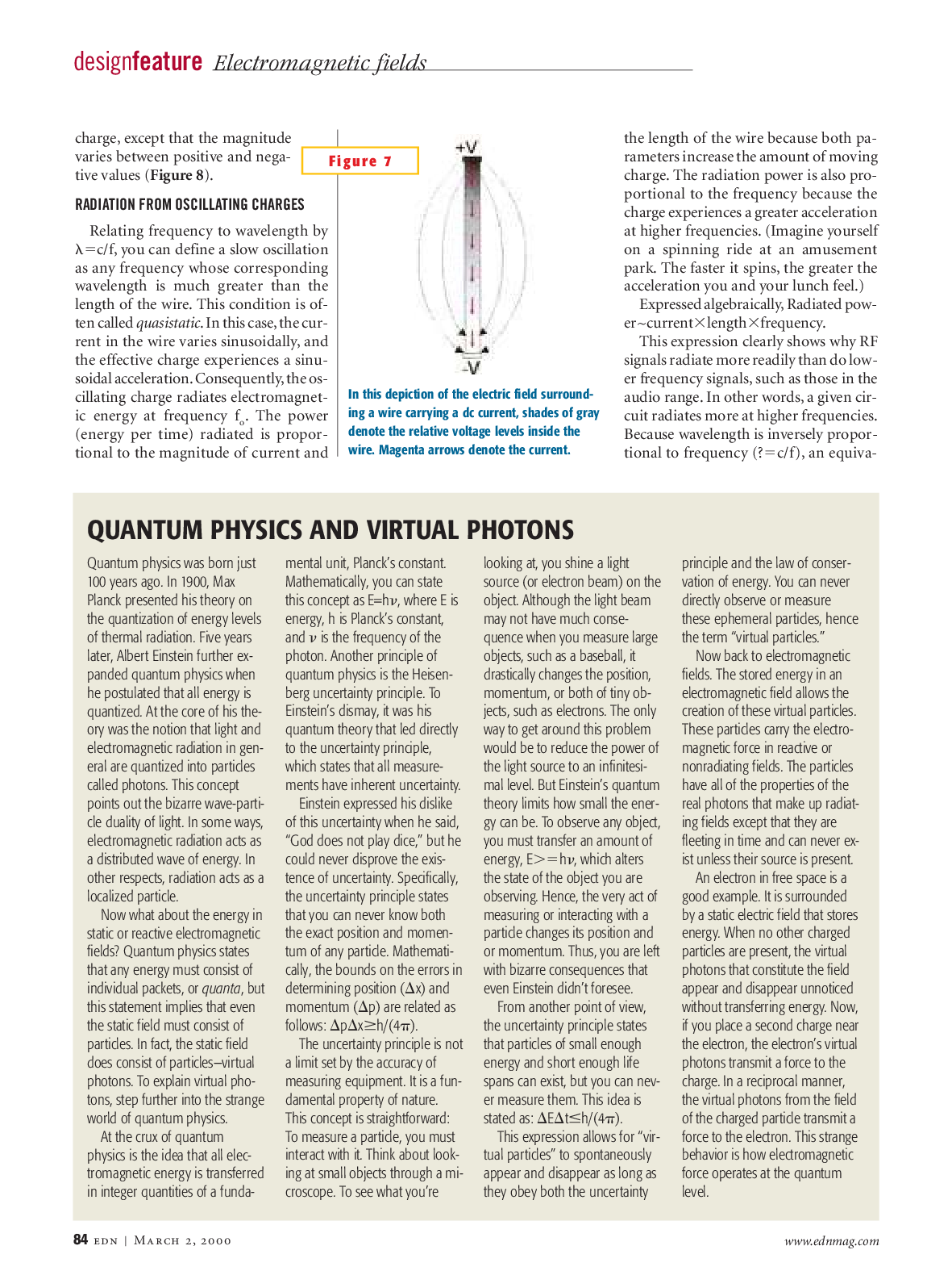
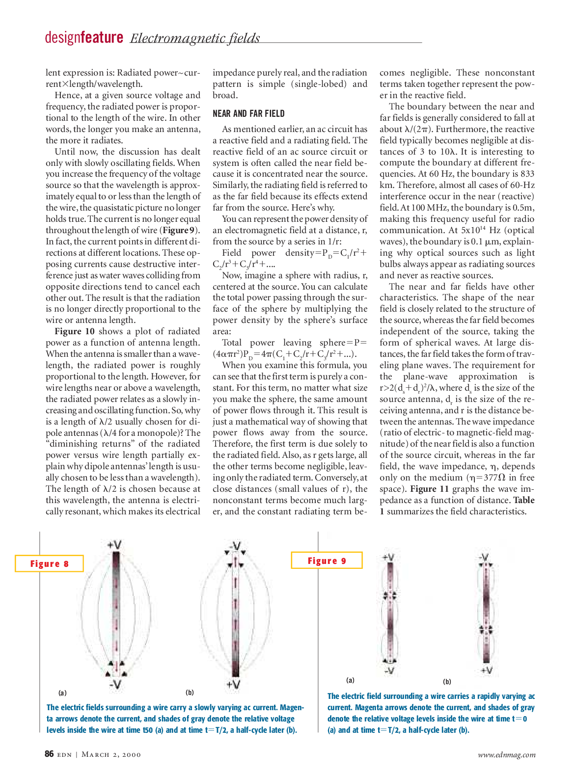
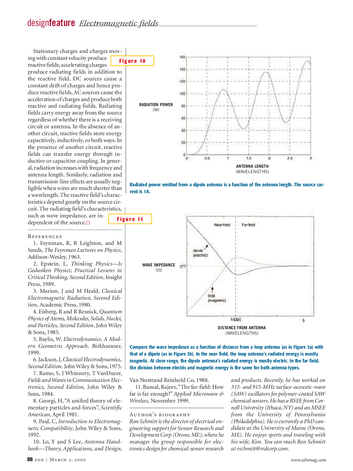
Just as for any impedance, the real part of the impedance transforms the electrical energy into energy in some other domain. In an ordinary resistor the power lost in the resistive component is transferred into heat; in an antenna it is transmitted. The following paper gives a nice introduction into the physics behind antennas; the paper is included with permission from Aspencore / EDNmag.
A dipole antenna is the most basic antenna; the construction of such a general dipole antenna is shown in Figure 11.1. The exact mathematical analysis is out of the scope of this book: only the basics of radio frequency circuits are dealt with therefore knowing basic electrical properties of simple antennas is sufficient. This section therefore only presents some formulas to be able to calculate some electrical properties.
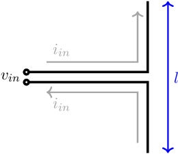
Calculating this can be done using the following set of equations [10], in case you’d be interested or if you want to get a numerical value. The impedance of the antenna connector is related to the “internal impedances” as follows:
The constants and are the wire thickness respectively the free space impedance for an EM-wave In vacuum or air, the radiation resistance of a half-wave dipole antenna equals . If the antenna shows no other significant resistive losses due to e.g. Ohmic losses in the antenna, then the radiation resistance is equal to the resistance of the antenna as a whole.
The impedance of an antenna consists of a resistance and a reactance (inductive or capacitive). For a half wave dipole, the antenna thickness does not seem to be of importance and its reactance in vacuum or air is . For other antenna lengths the relation is dependent on the thickness of the antenna. For the half wave dipole the reactance is — as you can see from the equation — positive for certain values of , and negative for other values. It might seem scary, a negative reactance, but it isn’t. As you know, the impedances of reactive elements are
thus a positive corresponds to an inductance and a negative to a capacitance.
The impedance of a dipole antenna as seen from a driving circuit is shown in Figure 11.2. This figure shows the impedance on the antenna feedpoint as a function of the ratio between antenna length and the wavelength , separating the real and reactive part of the antenna impedance. The figure shows that the antenna impedance can vary between low and high resistance, with a capacitive or inductive series reactance, as a function of the ratio .
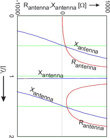
The EM-propagation speed in the antenna is about equal to the speed of light in vacuum from which it follows that for a signal frequency , . Consequently, the x-axis variable in Figure 11.2 is proportional to the signal frequency.
In circuit simulations of transmit (or receive) systems, the impedance of antennas should be taken into account properly. Figure 11.2 shows that the dipole behaves as a system with multiple resonances, at integer multiples of . For quick and not-too-dirty simulations, it may be sufficient to model the antenna at only a few frequencies of interest, modelling the DC-behavior (open for a dipole) and modelling at the transmit frequency (a series construction of a resistor and a reactance, see Figure 11.2).
A monopole is just half of a dipole antenna plus a ground plane. A dipole antenna is symmetrical: it is driven at the center and both halves do exactly the same thing concerning the radiation, impedance and some other stuff. This implies that we can identify a symmetry plane in a dipole. Having a symmetry plane in a symmetrically driven structure results in having no net signal at that symmetry plane. This allows us to put a grounded plane at that symmetry plane. If this symmetry plane is sufficiently large, then half of the dipole — the upper half or the lower half — can be removed without the remaining part noticing that (electrically)62 . T Hence, the differences between a dipole and a monopole are small:
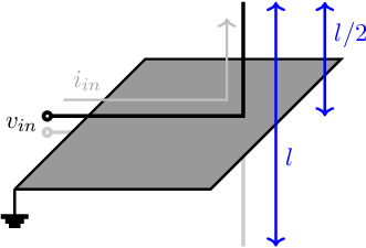
The equivalent of, for instance, a half wave dipole, is now a quarter wave monopole, with:
| half wave dipole | quarter wave monopole | |
| length | ||
We can keep on talking about antennas just about forever, but for this introductory course on electronics, that would not be very useful. However, it is useful to get acquainted with a few concepts concerning the antenna: the most important ones are discussed below.
Directivity and gain The terms directivity and gain of an antenna are often mixed up. The directivity of an antenna gives a measure of how well the antenna is capable of bundling its radiation to a specific direction. It doesn’t matter whether or not it is the transmit or receive antenna, since .
a dipole and monopole antenna are symmetric in a (2-dimensional) plane perpendicular to the arm(s). This implies that there is no reason whatsoever that in that plane the radiation in a specific direction is different from that in another direction. As a result, monopole and dipole antennas transmit and receive omnidirectionally perpendicular to the antenna arms.
Note that the receive and transmit power in the direction of the arms is low to zero, due to the same symmetry. sufficiently far away from the antenna then the radiated or received field adds destructively.
Numerically, the directivity or gain of an antenna give the ratio of transmitting power in one specific direction, related to the transmitting power of the isotropic antenna:
where the value of is usually given in : the gain or directivity compared to an isotropic antenna. The gain or directivity of a dipole antenna is . Antennae with a high directivity (or gain) radiate and receive mainly a narrow beam. Antennas that receive signals from many directions (almost) equally well have, by definition, a low gain and low directivity.