0 Preparatory knowledge

It is assumed that you already have some basic knowledge of electronic components, electronic circuit analysis and of mathematics. Nonetheless, a short recap is presented in this chapter. Also, there are multiple notations and symbols around for signals and components. This book sticks mainly to the European style. These notational things and the symbols are also summarized in this chapter.

0.1 Notation

This book uses a consistent notation for components and signals:

0.2 Linear components

Simple electronic networks are composed of linear components; the element equations and impedances of these are listed below.

 
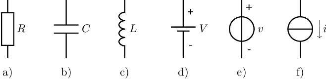
The symbols for the components above, as used in this book, are presented in figures 0.1a to c. Often a general impedance is used, rather than an impedance specifically for capacitors, inductors or resistors. In that case, the symbol for a resistor is used with a notation that indicates that it is an impedance: $Z_C$, $Z_R$, $Z_L$ or $Z_x$. In this reader the US-style wire wound resistor symbol (the zigzag one) is not used.

0.3 Independent sources

There are two basic types of independent sources: an independent voltage source and an independent current source. Usually, the term “independent” is dropped for simplicity.

The voltage source forces a voltage difference across its terminals, independent of the current that will flow due to that voltage. Hence, a voltage source can either deliver or dissipate energy. In this book, we will encounter two different independent voltage sources: the DC-voltage source (shown in Figure 0.1d) and the general voltage source (figure 0.1e).

The current source, shown in 0.1f, forces a current through its terminals. This current is independent of the voltage across its terminals. This book does not make any symbolic distinction between various current sources, DC, AC, independent or controlled.

0.4 Controlled or dependent sources

Circuits that have power gain are usually modelled using controlled voltage sources and/or controlled current sources, shown symbolically in figures 0.1e and f. The value of a source describes whether it is controlled or independent: e.g. a value $I_A$ corresponds to a DC-current source, while a value like $g_m\cdot v_{\mathit{in}}$ corresponds to a (here voltage) controlled current source.

0.5 Kirchhoff’s current and voltage laws

Kirchhoff’s voltage law (KVL) and Kirchhoff’s current law (KCL), formulated in 1845 by Gustav Kirchhoff, give elementary relations for electronic circuits¹ . Kirchhoff’s laws state that the total voltage drop in any mesh equals 0 V, and that no current can appear or disappear from nodes: ${\sum <!--\; FUNCTION\; APPLICATION\; -->}_{\mathit{mesh}}{v}_n=0$ and ${\sum <!--\; FUNCTION\; APPLICATION\; -->}_{\mathit{node}}{i}_n=0$.

In essence, the current and voltage laws are nothing more or less than the two most basic laws of (simple) physics: the laws of conservation of matter and conservation of energy.

As a short explanation: if you apply the law of conservation of matter to the particles we call electrons, you obtain Kirchhoff’s current law: electrons do not disappear or appear at random and hence the summed current into any node is zero. Furthermore, electrons have some level of energy, which is expressed in electronvolts [eV]. In electronics, we usually work with a large number of electrons (a Coulomb), which results in the unit of Volt [V]. Since electrons do not (dis)appear at random and energy does not either, the voltage drop in any mesh must equal 0 V.

0.6 Superposition

In any circuit, the voltage on a node (or the current in a branch) is resulting from the contribution of all sources in that circuit. However, calculating the voltage at some node in a circuit due to all sources simultaneously can be a lot of work.

With linear circuits, a voltage or current can be calculated much more easily by calculating the contribution of every source separately and finally summing all these contributions. This method is called superposition; it is one of the most powerful tools available for linear circuit analysis. The underlying idea is that a complex problem is separated into small problems in a very efficient way² .

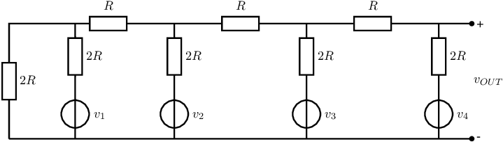
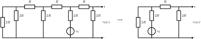
A good example of a circuit that can be easily analyzed using superposition, but quite difficult without superposition, is the R-2R-ladder circuit, shown in Figure 0.2.

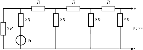
The output voltage as a function of the four independent sources is easily obtained if we calculate the separate contributions of all the independent sources. For the given circuit, we would have to do this four times. Calculating (only) the contribution of $v_1$, the circuit in Figure 0.2 can be redrawn as shown below. For this circuit it can be derived that $v_{\mathit{OUT}}(v_1)=\frac{1}{16}\cdot v_1$.

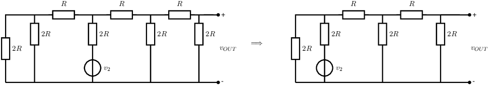
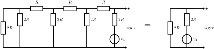
Calculating (only) the contribution of $v_2$, the circuit in Figure 0.2 can be redrawn as shown in Figure 0.4. For this circuit it can be derived that $v_{\mathit{OUT}}(v_2)=\frac{1}{8}\cdot v_2$. Similarly, the contribution of (only) $v_3$, follows from the Figure 0.5. In this figure, the original situation is shown on the left, while the simplified (redrawn) equivalent is depicted on the right hand side. For this circuit it can be derived that $v_{\mathit{OUT}}(v_2)=\frac{1}{4}\cdot v_3$. Lastly, the contribution of (only) $v_4$ to $v_{\mathit{out}}$ can be derived from the actual and simplified equivalent circuits in Figure 0.6 yielding $v_{\mathit{OUT}}(v_2)=\frac{1}{2}\cdot v_4$.

Summarizing these findings yields

This type of circuit is sometimes used to convert digital signals — setting $v_n$ either to 0 or to a well defined constant voltage dependent on (here) 4 bit digital data — to analog signals.

This example also shows that superposition and simplifying circuits whenever possible significantly reduces computational complexity: it leads to a ”divide and conquer”-strategy that usually enables many possible simplifications that bottom line reduce the amount of cumbersome calculations.

0.7 Advanced superposition

In most textbooks, superposition is formulated only for independent sources and it may appear that it does not hold for dependent (controlled) sources or for circuits that contain dependent sources. This is wrong! In the analysis of circuits, you can calculate the contribution of any linearly dependent source exactly the same way you’d do it for an independent source. The trick is that at some stage — preferably at the end of the calculations to limit the amount of work for you — you have to define the linearly dependent voltage or current for the controlled sources. It does not matter at all whether this value is independent or linearly dependent.

0.8 Thévenin and Norton equivalents

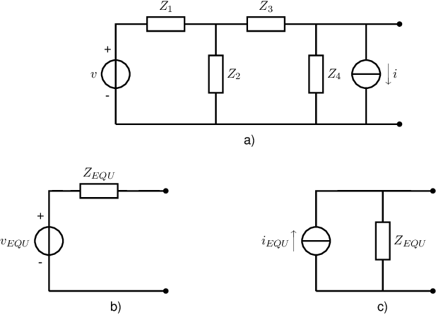
The electrical behavior of every linear circuit can be modelled as a single source and a single impedance. This can easily be seen using the definition of linear circuits, stating that linear I-V behavior can be described by a linear relation. Furthermore, any linear function is uniquely defined by any two (non-coinciding) points satisfying that function. In linear circuits, it is convenient to choose the points where the load is $Z=0\mathrm{\Omega }$ and $Z\to \infty \mathrm{\Omega }$.

From this, a simple equivalent model can be constructed with just one source and one impedance. If the equivalent uses a current source then we call it a Norton equivalent, while a model with a voltage source is called a Thévenin equivalent. Both are named after their discoverers, respectively in 1883 [1] and 1926 [2]³ .

The circuit in Figure 0.7a has its Thévenin and Norton equivalents shown in, respectively, Figures 0.7b and c. The open circuit voltage and short circuit current for this example are:

According to Ohm’s law, the following equivalent circuits hold:

0.9 Linear networks and signals

A linear network consists of linear components: resistors (with an instantaneous linear relation between voltage and current), capacitors and inductors (with an integral or differential relation between $v$ and $i$). The input source can either be a current source or a voltage source.

One of the most useful characteristics of a linear circuit is the fact that the input signal emerges undistorted at the output. This might seem counter intuitive: if we input for example a square wave into an arbitrary linear circuit, the output signal is in general not a square wave - the circuit may appear to be distorting the shape of the input signal. The circuit however is linear and is not distorting a specific class of signals, usually sine waves, and the input signal can be viewed as a summation of sine waves that individually remains undistorted, but that individually may get a different phase or amplitude. After summing these individually undistorted sine waves that all have experienced different phase shifts and gain, the sum of these may have a different shape than the input signal. Still, this is linear!

The types of signals where the output signal is a shifted and scaled version of the input signal $s$, are those that satisfy the following mathematical relation:

Signals that satisfy this are $\mathit{sin}(\mathit{\omega t}+\varphi )$ and $e^{(a+\mathit{jb})\cdot t}$: harmonic and exponential signals. Euler showed [3] that these two types of signals are closely related⁴ : $e^{\mathit{jb}\cdot t}$ is a rotating unit vector in the complex plane with angle $\mathit{bt}$. The representation of this on the real axis is $\mathit{cos}(\mathit{bt})$, while the imaginary part is $j\cdot \mathit{sin}(\mathit{bt})$. From this, it follows that:

In this book we assume the sine waves as these allow easier interpretation, calculation, simulation and measurement of circuit behaviour in terms of gain and phase shift (per sine wave).

0.10 Complex impedances

Assuming a sinusoidal signal, it is now straightforward to derive the impedance of reactive elements. For a capacitor it follows (assuming a sinusoidal signal) that:

Similarly, for an inductor:

It may appear weird that the ratio of a $\mathit{sin}(\mathit{\omega t})$ and a shifted $\mathit{sin}(\mathit{\omega t}+\varphi )$ is rewritten into a complex number.; weird that e.g. $\mathit{sin}(\mathit{\omega t}+90^{\circ })∕\mathit{sin}(\mathit{\omega t})=j$ instead of being $\mathit{tan}(\mathit{\omega t})$. The reason is that in the frequency domain it is all about the magnitude and the phase of harmonic signals, and the phase of the $\mathit{sin}(\mathit{\omega t}+90^{\circ })$ leads that of $\mathit{sin}(\mathit{\omega t})$ by $90^{\circ }$ while the magnitudes are identical. A complex number that captures this is the number having modulus 1 and argument $90^{\circ }$ which is the complex number $j$.

0.11 Fourier transformations

The basic signals used to analyze linear circuits — the sine waves — have a close correlation to Fourier analysis. Fourier stated [4] that every periodic signal $f(x)$ can be written as an infinite sum of harmonic signals:

Using a number of goniometric relations, the Fourier transformation of a signal is obtained. The relevant equations here are:

The first two relations state that the average of a harmonic signal equals 0. The third relation states that the sum of a sine and a cosine with the same argument can be written as one harmonic function with that argument and a phase shift. The fourth relation is crucial: the product of two harmonics equals the sum of two harmonics, one with the difference between the arguments, the other with the sum of the arguments. From the first three relations, it immediately follows that if a periodic signal with angular frequency $\omega$ can be written as the sum of harmonics, then those harmonics must have angular frequencies which are an integer multiple of the angular frequency of the original signal. Now, a new relation can be written:

Note that the $a_0$-term corresponds to the $0^{\mathit{th}}$ harmonic, or in fact the $a_0\cdot \mathit{cos}(0)$ term. The above relation can already be used to perform Fourier transformations: all $a_n$ terms and all ${\varphi }_n$ factors would have to be determined. However, in general, determining the ${\varphi }_n$ factors can be very difficult. Using the $3^{\mathit{rd}}$ goniometric relation, this yields the most widely used Fourier formula:

From the fourth goniometric relation, together with the first two, the relation to determine $a_n$ and $b_n$ can be derived quite easily:

The Laplace transformations are closely correlated to Fourier transformations: the most important “differences” include the use of $e^{\mathit{jx}}$ instead of $\mathit{sin}(x)$ and $\mathit{cos}(x)$ and using $s$ instead of $\mathit{j\omega }$. In this book, basic knowledge of Fourier series is assumed, as this is used implicitly in many chapters. Although Laplace is very useful for e.g. stability analyses and calculating time responses it is not used in this book.

0.12 Differential equations

It is convenient to analyze circuits in the frequency domain using complex impedances, which is however only allowed for linear circuit because of the linear (Fourier) transform that underlies complex impedances. Typically circuits that are sufficiently linear (i.e. have sufficiently low distortion for the signals that are used in the analysis) are analyzed in the frequency domain. Then the resulting small inaccuracies are accepted. Moreover, to simplify the analyses the circuits are usually upfront modelled as being linear. This approach will be followed later in this book to simplify analyses significantly.

From a fundamental point of view non-linear circuits cannot be analyzed in frequency domain. If a circuit is very non-linear or switching, typically linearisation is not allowed and any sine wave would be very much distorted in the circuit. Then complex impedances — assuming single sine waves in a circuit — cannot be used. As only resort, time-domain element equations must be used and these require time domain analyses, usually in the form of differential equations. Below is a short summary for $1^{\mathit{st}}$ and $2^{\mathit{nd}}$ order differential equations, here written as respectively

It is evident from this that signal $x(t)$ has a derivative that has the same shape as the signal itself, i.e. either exponential or harmonic. Including the demand for an arbitrary phase shift in the shape, the only valid shape is the exponential shape: the derivative of a sine wave has a fixed phase shift with respect to the sine wave itself. The easiest solving method⁵ is to substitute the most general form and solve the missing parameters for the homogeneous solution:

Clearly there is just one solution for first-order differential equations, and two for second-order differential equations (and yes, $n$ for an $n^{\mathit{th}}$ order differential equation). These two solutions can be complex, in which case an (exponentially increasing or decreasing) harmonic solution results:

When there are only real solutions, the output is the sum of two exponential functions. The particular solution, where $D$ is also implemented, has to be solved next. This usually takes some tricks⁶ . From all initial conditions, the rest of the parameters can usually be determined.

0.13 Circuit analysis methods

A number of circuit analysis methods for (linear) electronic circuits is well known. The most common methods are the nodal analysis and the mesh analysis; in this book, we will mostly be using the brute force approach . All these methods are very systematic, and while the first two are very well suited for implementation in software, the third method gives more insight (although it is difficult to automate in software).

• With the nodal analysis, the total current into every node of a circuit is equated to zero. This is hence implementing Kirchhoff’s current law.
  For easy calculation of the currents, passive components are included by their admittances instead of their impedances and only current sources are allowed in the circuit. Any voltage source then needs to be first replaced by its Norton equivalent. If this method is performed properly, a network of $N$ nodes gives a set of $N$ independent equations, which can be solved to give all voltages. For e.g. the circuit in Fig. 0.8, having 3 nodes, the 3 equations are:

  

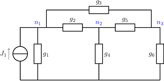
  $$\begin{array}{llll}\hfill v_1\cdot (g_1+g_2+g_3)-v_2\cdot g_2-v_3\cdot g_3& =J_1& \hfill & \\ \hfill -v_1\cdot g_2+v_2\cdot (g_2+g_4+g_5)-v_3\cdot g_5& =0& \hfill & \\ \hfill -v_1\cdot g_3-v_2\cdot g_5+v_3\cdot (g_3+g_5+g_6)& =0& \hfill & \end{array}$$ Solving this set of equations can be done by hand, for example using Gaussian elimination. This set of equations can also be solved easily in software for which the set of equations is written in matrix-form:

  $$\left[\begin{array}{ccc}\hfill g_1+g_2+g_3\hfill & \hfill -g_2\hfill & \hfill -g_3\hfill \\ \hfill -g_2\hfill & \hfill g_2+g_4+g_5\hfill & \hfill -g_5\hfill \end{array}\right]\left[\begin{array}{c}\hfill v_1\hfill \\ \hfill v_2\hfill \end{array}\right]=\left[\begin{array}{c}\hfill J_1\hfill \\ \hfill 0\hfill \end{array}\right]$$

  Solving this equation numerically can be done easily using matrix inversion. Matrix inversion in software is usually implemented via LU-decomposition, Gaussian elimination and backward substitution. You can also do it by hand, which is boring and non-insightful. Sorry to inform you about that. CPUs do like it a lot though and are happy to do it.

• The mesh analysis is based on Kirchhoff’s voltage law and therefore equates the summed voltage in any mesh in a circuit to zero. Just as with the nodal analysis, a set of equations is formulated that has to be solved. Since the mesh analysis uses voltages, current sources must first be replaced by their Thévenin equivalents. The circuit in 0.9 then gives:

  

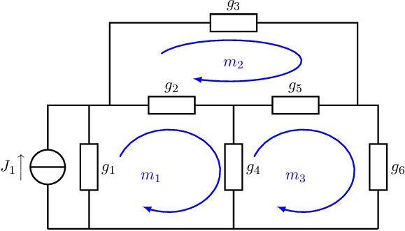
  $$\begin{array}{llll}\hfill i_1\cdot (Z_1+Z_2+Z4)-i_2\cdot Z_2-i_3\cdot Z_4& =E_1& \hfill & \\ \hfill -i_1\cdot Z_2+i_2\cdot (Z_2+Z_3+Z_5)-i_3\cdot Z_5& =0& \hfill & \\ \hfill -i_1\cdot Z_4-i_2\cdot Z_5+i_3\cdot (Z_4+Z_5+Z_6)& =0& \hfill & \end{array}$$ or equivalently in matrix form:

  $$\left[\begin{array}{ccc}\hfill Z_1+Z_2+Z4\hfill & \hfill -Z_2\hfill & \hfill -Z_4\hfill \\ \hfill -Z_2\hfill & \hfill Z_2+Z_3+Z_5\hfill & \hfill -Z_5\hfill \end{array}\right]\left[\begin{array}{c}\hfill i_1\hfill \\ \hfill i_2\hfill \end{array}\right]=\left[\begin{array}{c}\hfill E_1\hfill \\ \hfill 0\hfill \end{array}\right]$$

  This can again be solved with Gaussian elimination and backward substitution: fancy terms for simply working in a systematic manner to solve a set of linear equations. Just as with the nodal analysis you can do it by hand, but a computer is much better at it. To make it worse, you probably do not get a lot of insight from doing these matrix inversions by hand.

• The modified nodal analysis combines nodal and mesh analysis in one go. In this way both independent voltage sources and current sources and any (linear) circuit component can be handled in one set of equations (or matrix). This modified nodal analysis is typically used in computer programs to solve circuit equations. By hand it is really a lot of tedious work.

• The brute force approach is also a very systematic way to derive relations (transfer functions, impedances, ...) aiming at relatively small circuit and aiming at hand derivations.

  The starting point of the brute force approach is the target result in its most (trivial) basic form. Solving that target result is done by iteratively solving parts of that most basic form until everything is known. Via subsequently back substitution the full (non-trivial) form of the end result is obtained. Advantages of this brute force approach is that this method inherently only takes parts of the problem (circuit) into account that are relevant for your end result: all non-relevant things are inherently ignored. Another advantage is that it tends to provide insight into solving the problem.

  The brute force approach uses (for electronic circuits) Kirchhoff’s voltage law, Kirchhoff’s current law, and the element equations, whichever comes in handy at that instant. In a circuit with $N_m$ voltage meshes, $N_k$ nodes and $N_c$ electronic components, obtaining the answer takes a maximum of $(N_m+N_k+N_c)$ derivation steps, and another $(N_m+N_k+N_c)$ substitution steps. If some parts of the circuit are not relevant to get your end result everything from those parts do not end up in the derivation! For small circuits this method if efficient. This brute force approach is used throughout this book.

  brute force approach - step 1
  The first equation that should be formulated in the brute force approach is the target relation, the desired outcome in its most basic form. For example, if a voltage transfer $H$ is aimed at, then the first statement would be a small elaboration (or specification) of that target relation:

  $$H=\frac{v_{\mathit{OUT}}}{v_{\mathit{IN}}}$$

  brute force approach - step 2
  Next, every unknown on the right hand side of the relation must be solved iteratively using KVL, KCL or an element equation. In this, iterative solving multiple — equally correct — choices can be made. For example if a current must be solved, this can usually be done using KCL or by an element equation. There is no preference in which one to choose as long as you keep in mind that (just as in any mathematical derivation) the restriction is that every relation can be used only once⁷ .

  In iteratively solving equations, it is important to recognize that all variables for which an expression has already been derived (and hence, is on the left hand side of a “=”-symbol) is known. For the transfer of the voltage from $E_1$ to $v_{n2}$ in Figure 0.9, we will get, for example:

  $$\begin{array}{llll}\hfill & H=\frac{v_{n2}}{v_{E_1}}& \hfill & \\ \hfill & v_{n2}=i_{z4}\cdot Z_4(\mathit{EE})& \hfill & \\ \hfill & i_{z4}=i_{z2}+i_{z5}(\mathit{KCL})& \hfill & \\ \hfill & i_{z2}=\frac{v_{n1}-v_{n2}}{Z_2}(\mathit{EE})& \hfill & \\ \hfill & i_{z5}=\frac{v_{n3}-v_{n2}}{Z_5}(\mathit{EE})& \hfill & \\ \hfill & v_{n1}=v_{E1}-v_{z1}(\mathit{KV}L)& \hfill & \\ \hfill & \mathrm{\text{(no need to solve }}{v}_{n2}\mathrm{\text{ - already defined!)}}& \hfill & \\ \hfill & v_{n3}=i_{z6}\cdot Z_6(\mathit{EE})& \hfill & \\ \hfill & v_{z1}=Z_1\cdot (i_{z2}+i_{z3})(\mathit{EE})& \hfill & \\ \hfill & i_{z6}=-i_{z5}+i_{z3}(\mathit{KCL})& \hfill & \\ \hfill & i_{z3}=\frac{v_{n1}-v_{n3}}{Z_3}(\mathit{EE})& \hfill & \end{array}$$

  brute force approach - step 3
  Back substituting these equations gives a non-trivial equation for the desired answer. It seems like a lot of cumbersome work, but other methods need at least as much (or even more) effort for relatively small circuits such as used in this book.

  Below, a part of the back substitution is presented. While calculating the $v_{n3}$, we get an expression that is a function of $v_{n3}$. This indicates that there are loops (feedback paths) in the circuits. The best way to continue is to separate the variables, as shown below⁸ .

  $$\begin{array}{llll}\hfill & i_{z6}=-i_{z5}+\frac{v_{n1}-v_{n3}}{Z_3}& \hfill & \\ \hfill & v_{z1}=Z_1\cdot (i_{z2}+\frac{v_{n1}-v_{n3}}{Z_3})& \hfill & \\ \hfill & v_{n3}=-i_{z5}\cdot Z_6+\frac{v_{n1}-v_{n3}}{Z_3}\cdot Z_6⟺\mathrm{\text{ (separate variables)}}& \hfill & \\ \hfill & v_{n3}(1+Z_6∕Z_3)=-i_{z5}\cdot Z_6+\frac{v_{n1}}{Z_3}\cdot Z_6⟺& \hfill & \\ \hfill & v_{n3}=-i_{z5}\cdot \frac{Z_6{Z}_3}{Z_3+Z_6}+\frac{v_{n1}}{Z_3+Z_6}\cdot Z_6& \hfill & \end{array}$$

  Continuing the back substitution yields the desired answer. Smaller circuits or circuits without loops (here, for example with $Z_3$), require less work. The brute force approach will be used for small circuits in this book. Larger and more complex circuits will be divided into subcircuits. Then after analyzing these subcircuits, the overall result can be created from the results of the subcircuits. Analyzing large circuits by hand typically is not useful as it would yield large equations that are too hard to understand and hence are meaningless.

  $$\begin{array}{llll}\hfill & v_{n1}=...& \hfill & \\ \hfill & i_{z2}=...& \hfill & \\ \hfill & i_{z5}=...& \hfill & \\ \hfill & i_{z4}=...& \hfill & \\ \hfill & v_{n2}=...& \hfill & \\ \hfill & H=...& \hfill & \end{array}$$

  brute force approach - wrap up
  With the brute force approach you are iteratively working toward solving for one a specific answer, while your method is based on the divide and conquer method and only uses the most basic equations. With the brute force approach a complex problem — e.g. calculating some transfer function or impedance — is divided into many very simple problems — e.g. element equations, KCL, KVL — which are combined to get the complete answer. This method is efficient in terms of insight and complexity for small circuits (only) such as used in this book.

0.14 Transfer functions

In electronics, we often want to get relations between the input signal and something which is a consequence of that signal. Usually this consequence is an output signal, meaning that we often have to find a transfer function. Other meaningful relations include those for the input and output impedance of an electronic circuit:

To analyze, sketch or interpret these transfer functions or impedances it is usually convenient to rewrite the original function as (a product or sum of) standard forms. There are several standard forms; for a low-pass-like transfer function:

The first form corresponds to an integrator, which is just a limit case of the second form. The second and third forms are identical, and have a first-order characteristic; the fourth form has a second-order characteristic. High-pass characteristics can be obtained from low-pass functions, using:

From this it follows that:

The order of any transfer function is simply equal to the highest power of $\omega$. Every normal transfer function, of arbitrary power, can be written as the product of first and second-order functions. Knowing the three basic standard forms for low-pass characteristics by heart and being able to do some basic manipulations pretty much covers everything you will ever need to visualize transfer functions or impedances as a function of frequency.

0.15 Bode plots

A Bode plot is a convenient method for presenting the behaviour of a (linear) circuit; this is done by plotting the magnitude and phase shift of a transfer function as a function of the frequency. Here, the magnitude and frequency are plotted on a logarithmic scale, which proves to be very convenient⁹ . Before we dive into Bode diagrams, we first repeat a number of mathematical logarithmic rules:

In words:

• the product of two values on a logarithmic scale equals the sum of those two values.
• a relation $x=y^z$ on a log-log scale gives a straight line with a slope of $z$; where $z$ can be any real number.
• the sum of 2 values, as approximation, equals the largest of the two values on a logarithmic scale. Only if these numbers are more or less the same size, this rule does not apply.

To calculate the argument of a (complex) transfer function, standard rules for complex numbers can be used. The most important one that is used for Bode plots is that the angle (or argument or phase) of the product of two complex numbers equals the sum of the angles of the individual numbers: $\angle (A\cdot B)=\mathit{\angle A}+\mathit{\angle B}$.

Bode plot for first order transfer functions

For example, the standard form of a first-order low-pass transfer function is $H(\mathit{j\omega })=H(0)\cdot \frac{1}{1+j\frac{\omega }{{\omega }_0}}$. Assuming for simplicity reasons only $H(0)>0$,

• for $\omega <<{\omega }_0$,

  $$H(\mathit{j\omega })=H(0)\cdot \frac{1}{1+j\frac{\omega }{{\omega }_0}}\approx H(0)$$

  and consequently the transfer function almost equals $H(0)$, with a phase shift of $0^{\circ }$. Note that for negative $H(0)$ the $\pm 180^{\circ }$ phase shift due to the negative sign should also be taken into account.

• for $\omega >>{\omega }_0$,

  $$H(\mathit{j\omega })=H(0)\cdot \frac{1}{1+j\frac{\omega }{{\omega }_0}}\approx -jH(0){\omega }_0\cdot {\omega }^{-1}$$

  yielding a modulus equal to$H(0){\omega }_0\cdot {\omega }^{-1}$ with a phase shift of $-90^{\circ }$. Due to the proportionality of the modulus to ${\omega }^{-1}$, the magnitude part of a Bode plot shows a constant slope equal to -1 (plotting $\mathit{log}(|H(\mathit{j\omega })|)$ or -20dB/decade (plotting the magnitude in dB).

• for $\omega ={\omega }_0$,

  $$H(j{\omega }_0)=H(0)\cdot \frac{1}{1+j}$$

  which corresponds to a modulus $H(0)∕\sqrt{2}$ with a phase shift equal to $-45^{\circ }$. Expressed in dB, the factor $\sqrt{2}$ corresponds to -3dB. Drawing the magnitude part of the Bode plot asymptotically, the 2 asymptotes touch at $\omega ={\omega }_0$ and $H(j{\omega }_0)=H(0)$.

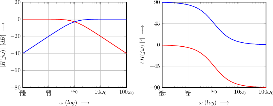
Using this, the Bode plot of a first order low pass transfer function $H(\mathit{j\omega })=H(0)\cdot \frac{1}{1+j\frac{\omega }{{\omega }_0}}$ is as shown in Figure 0.10. The corresponding curves for this low-pass transfer function are shown in red. The curves for a first order high pass transfer function $H(\mathit{j\omega })=H(0)\cdot \frac{j\frac{\omega }{{\omega }_0}}{1+j\frac{\omega }{{\omega }_0}}$ are shown in blue.

Bode plot for second order low pass transfer functions

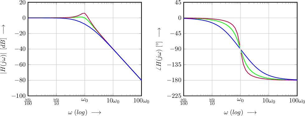
A similar analysis/construction can be done to create a Bode plot for second order transfer functions. Below, this is done for low pass transfer functions, for a few different values for Q. Again a positive $H(0)$ is assumed for simplicity reasons.

• for $\omega <<{\omega }_0$,

  $$H(\mathit{j\omega })=H(0)\cdot \frac{1}{1+j\frac{\omega }{{\omega }_0\cdot Q}+j^2\frac{{\omega }^2}{{\omega }_0^2}}\approx H(0)$$

  and consequently the transfer function almost equals $H(0)$, with a phase shift of $0^{\circ }$.

• for $\omega >>{\omega }_0$,

  $$H(\mathit{j\omega })=H(0)\cdot \frac{1}{1+j\frac{\omega }{{\omega }_0\cdot Q}+j^2\frac{{\omega }^2}{{\omega }_0^2}}\approx -H(0){\omega }_0^2\cdot {\omega }^{-2}$$

  yielding a modulus equal to$H(0){\omega }_0^2\cdot {\omega }^{-2}$ with a phase shift of $-180^{\circ }$. Due to the proportionality of the modulus to ${\omega }^{-2}$, the magnitude part of a Bode plot shows a constant slope equal to -2 (plotting $\mathit{log}(|H(\mathit{j\omega })|)$ or -40dB/decade (plotting the magnitude in dB).

• for $\omega ={\omega }_0$,

  $$H(j{\omega }_0)=H(0)\cdot -jQ$$

  which corresponds to a modulus $H(0)\cdot Q$ with a phase shift equal to $-90^{\circ }$.

Using this, the Bode plot of a second order low pass transfer functions with $Q=0.4$ (blue curves), $Q=1$ (green curves) and $Q=2$ (purple curves) are shown in Figure 0.11.

Bode plots for other transfer functions

In most electronic systems, transfer functions are not first order or second order. A generic transfer function can be decomposed into the product of first order (high pass or low-pass) and second order transfer functions (idem). Constructing a Bode plot of the product of (basic) transfer functions is quite simple which is due to the fact that fo two complex numbers $c_1$ and $c_2$,

Then, constructing a Bode plot of $H_{\mathit{total}}(\mathit{j\omega })=H_1(\mathit{j\omega })\cdot H_2(\mathit{j\omega })\cdot \dots$ can easily be done.

• Plot the curves of the $H_n(\mathit{j\omega })$ in the Bode plot.
• To get the magnitude part of the Bode plot of $H_{\mathit{total}}(\mathit{j\omega })$, just add the curves in the magnitude part of the Bode plot for all $H_n(\mathit{j\omega })$. This leverages the fact that adding on a log-scale corresponds to multiplication.
• To get the phase part of the Bode plot of $H_{\mathit{total}}(\mathit{j\omega })$, add the curves in the phase part of the Bode plot for all $H_n(\mathit{j\omega })$.

Done.

0.16 Calculations & mathematics

Calculations (or mathematics for more complicated calculations) is a necessity for describing something in an exact manner. Without calculations, there would only be vague statements like “if I change something here, then something changes over there” or “if I press here, it hurts there”. Those statements are completely useless! As in any sensible scientific field, in electronics we like to get sufficiently exact relations that are described in an exact language: mathematical terms. To refresh some basic math knowledge, this section reviews some of the most basic math rules. They may appear trivial but in the past number of years did not prove to be so.

0.17 The basics

The basis of almost all math is the equation, or a “=” with something on the left hand side, and something else on the right hand side. What those somethings are exactly is not important, but the two somethings are equal to each other in some way and probably have a different form.

These days, in elementary school, students do math with apples, pears and pizzas:

This is of course complete nonsense! Even if you would assume all pizzas to be of exactly the same size, shape and appearance (ingredients and their location), it would still depend on how you slice the pizza in half. It is possible to slice a pizza in half in, more or less, $\infty$ different directions, and if I cut the half pizzas in (0.1) in two different directions from full pizzas, then there is no way the two of them will be one complete pizza again, although it is suggested by (0.1)¹⁰ .

In electronics, our job is a little different: typically we use (integer) numbers of electrons, (a real number of) electrons per second or (real) energy per electron: with charge, or current and voltage. We might possibly add flux if we are talking about inductors, but the physics gets a bit more complicated since we would have to take relativity and Einstein into account. In general, we are dealing with matter that can easily be added, subtracted, divided and multiplied. The basics for doing math then is simply the equation:

often written in a somewhat different form:

It clearly states that the part left of the “=”-symbol is equal to the part on the right. More specific: its value is identical, not its form. Often, we would like to rewrite the equation to have something simple on the left hand side (we “read” from left to right) which is understandable (monthly pay, speed, impedance, ...) and a form on the right hand side that includes a bunch of variables. This is what is called an equation or relation: if you change something on the right hand side, something also changes on the left hand side, and vice versa. Such mathematical relations give the relation between different parameters and are very valuable in analyses and syntheses¹¹ .

0.18 Basic rules

The most basic rules for relations are formulated below. They only ensure that during manipulation the “=”-symbol is not violated.

• if you add something to the left hand side of an equation, you must also add that to the right hand side (and vice versa)
• if you multiply the left hand side of an equation, you must also multiply the right hand side by the same factor (and vice versa)
• you can add any 0 to either side of the equation
• you can multiply either side of the multiplication by 1

That’s it.

0.19 Basic math rules

In addition to the basic rules above, it is also assumed that the basic mathematical rules for exponential functions are known and can be applied by you. Also, the derivatives of some basic functions must be known by heart. If you remember how $e^{\mathit{something}}$ and harmonic signals (sine and cosine) are related, then you have enough knowledge to start off in this book. If you have some skill in manipulations with equations, can work in a structured way, have some perseverance and some confidence in yourself, then you should be just fine!

0.20 Simplifying relations

In this book relations will be derived frequently: mostly for impedances and transfer functions. Relations will be derived, since these relations will help you to analyze, understand, optimize and synthesize things. When deriving these equations, some skills in simplifying equations would come in handy. Simplifying equations boils down to using the basic rules in the previous section.

• using the equation ”something=something”
• multiplication by 1

The big challenge in the multiplication by 1 is in choosing the correct 1. For example the voltage transfer of a voltage divider out of a capacitor and a resistor can be derived to be:

which is an ugly expression, which can become more readable after multiplication by 1. Note that the relation does not change, only the form or appearance does. If you choose the correct 1, the relation gets nicer to read...

A parameter or signal may be a function of itself. For instance, the relation

looks nothing like a closed expression for $y$. The solution is obviously “separation of variables”, a trick which comes down to adding “something=something” to something¹² . A well chosen “something=something” gives:

Simplifying even further can be easily done by multiplying with a well chosen ”something=something”, like:

Hence, in order to simplify a relation, it is really importance to have mastered the multiplication table of 1 and to be able to use the equation $1=1$. This seems easy, but it usually proves to be very difficult.

0.21 Impedance matching and maximum power transfer

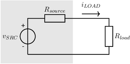
The power dissipated up in a load impedance $R_{\mathit{load}}$, using a source having a source impedance $R_{\mathit{source}}$ can straight forwardly be calculated. In this calculation, the notation detailed in section 0.1 is used where e.g. $V_{\mathit{src}}$ denoted the amplitude of voltage $v_{\mathit{SRC}}$. The maximum power in the load as a function of $R_{\mathit{load}}$ can be obtained by differentiation:

It follows that the power in the load is maximum if the load resistance is equal to the source resistance: $R_{\mathit{load}}=R_{\mathit{source}}$. In a similar way, the maximum power in the load for complex impedances is for $Z_{\mathit{load}}=Z_{\mathit{source}}^{\ast }$. A fairly simple result. But also a result that is only valid when designing the load impedance ans without any limitation in the signal source. In this book, the focus is however on designing oscillators and amplifiers that drive a load...

The optimum above is always true, since it is a mathematical truth. However, it assumes a fixed source impedance, no voltage or current limitation of the signal source and assumes that the load impedance is designed. Designing amplifiers that drive a load, the amplifier’s output voltage range, the amplifier’s output current range and the amplifier’s output impedance can be (and are) designed. Ensuring that the amplifier can supply a sufficient output voltage and output current, the maximum power into the load then follow from the following two (partial) derivatives:

from which it follows that

• the partial derivative $\partial P_{\mathit{load}}∕\partial R_{\mathit{source}}\le 0$ for every source voltage (amplitude) and combination of resistors. Hence, to obtain maximum power into the load, the output impedance of the amplifier $R_{\mathit{source}}$ must be as low as possible.
• the partial derivative $\partial P_{\mathit{load}}∕\partial V_{\mathit{src}}\ge 0$. Therefore, to obtain maximum power in the load, the voltage (amplitude) $V_{\mathit{src}}$ must be as large as possible,

If these two conditions are satisfied, then clearly the load and source impedances are not matched to achieve maximum output power. The upper limit in maximum power into the load for a given load impedance is then simply limited by the maximum output voltage OR by the maximum output current that can be provided simultaneously by the amplifier. This is worked out in more detail in section 11.14.

0.22 Solving exercises

Most problems can be tackled in the same general way.

1.

Understand the question, then try to specify it. For example, if you are asked for an output impedance, start writing something like:

$$z_{\mathit{out}}=?$$

or

$$z_{\mathit{out}}=\frac{\partial v_{\mathit{OUT}}}{\partial i_{\mathit{OUT}}}=\frac{v_{\mathit{out}}}{i_{\mathit{out}}}=?$$

This gives you a clear direction for the derivation. You can also check afterwards whether you actually calculated what you wanted to know.

2.

Make a drawing/schematic where all relevant items for this specific problem are presented. Leave out everything that is not important. You might need multiple drawings / schematics to obtain a final version. Putting something together quickly usually yields incorrect results or causes unnecessarily complex calculations.

3.

Work in a structured manner towards the answer. This can be done in several ways, some of which will be presented in this book.

4.

Verify your answer:

• Check whether it is actually an answer to the question.

• Check whether the dimensions (units) agree. If the dimensions are correct, then it might be the correct answer. Example:

  $z_{\mathit{out}}=\frac{R_o\left(1+i_d\cdot C_{\mathit{in}}\right)}{1+j\frac{\omega }{{\omega }_0}}$ must be wrong: $\mathrm{\Omega }\ne \frac{\frac{V}{A}\cdot \left(1+A\cdot \frac{\mathit{As}}{V}\right)}{1+1}$

  $z_{\mathit{out}}=\frac{R_o\left(1+\frac{i_d}{v_{\mathit{in}}\cdot \mathit{j\omega }{C}_{\mathit{in}}}\right)}{1+j\frac{\omega }{{\omega }_0}}$ can be correct: $\mathrm{\Omega }=\frac{\frac{V}{A}\left(1+\frac{A}{V\cdot 1∕s\cdot \frac{\mathit{As}}{V}}\right)}{1+1}$

• Check whether the equation passes the ‘test of extremes’ (fill in an extreme value which simplifies the problem, and reason whether or not this could be correct). Often 0 and $\infty$ are useful extremes. If you use the previous answer:

  $z_{\mathit{out}}\left(\omega =0\right)\to \infty$ and $z_{\mathit{out}}\left(\omega \to \infty \right)=0$

In addition, there are a number of issues which are useful to keep in mind. The exercises of any course can be solved; you don’t have to worry whether or not you have enough parameters. There even may be too many parameters within one exercise, just to let students think more and learn more.

In more complicated assignments, it is not always evident that you have enough data to actually calculate something. Before you start calculating, it might be useful to validate whether or not you are actually capable of calculating something in the first place. One approach for this is to use the fact that you need $n$ independent equations to solve $n$ variables. If you have less equations: be smart. If you have more equations or conditions: compromise!

Furthermore, it is always useful to work with variables, instead of numbers. Firstly you then make fewer mistakes and it allows to perform some basic sanity checks on your answer. Secondly, on tests, if you would make a minor mistake using variables that is a minor issue while it would be a direct and complete fail for numerical answers. Thirdly, relations can be (re)used and (fourthly) allow for synthesis.

When you work with variables, preferably use a divide and conquer strategy. Divide your problem in subproblems, solve these individually and construct the overall solution from these. This significantly reduces the amount of work (calculations) compared to directly calculating properties for a bigger system.

If you follow points 1 to 3, you are able to solve just about any problem, in electronics or otherwise. Point 4 is to verify your answer. By now, you might be wondering why there is nothing stated here about verification using the answer manual.

0.23 Verification using the answer manual

An answer manual is for most students (obviously not for you) useless, since it is typically used the wrong way: the example derivation is read along with the exercise which makes many students conclude that they would have been able to solve it themselves. However, actually being able to solve the problem and to understand the solution are two entirely different concepts.

The correct way to handle an answer manual, is:

• follow the four easy steps listed on the previous two pages

• After step 1:

  • “I do not know the answer”: great! If you would have known the answer immediately, it would have been a terrible question, since it would be too easy or focused on simply remembering stuff.
  • after 5 minutes of puzzling: first mutter how difficult this question is, then be happy that you are given the opportunity to learn something.

• After step 2-3 (and possibly 4):

  • solving the problem all by yourself (after puzzling, reading, puzzling, thinking, trying, $>$30 minutes). If you have not succeeded, ask someone (quite possibly a tutor) a question that pinpoints where and why you are stuck.

• When done:

  • if you are confident that your answer is correct, then verification using an answer manual is not necessary since you are confident. The only use would be that you see that your answer could have been written in another form. Since any relation can be written in an infinite number of different forms this is quite useless.
  • if you are not confident that your answer is correct, then verification is senseless because you would have had to continue until you’d had the confidence.

In essence, every answer manual is useless; Herman Finkers already stated “stories for in the fireplace” (freely translated) [5]. In the end, the only correct way of using an answer manual is not using it at all.

0.24 And finally...

Some useless knowledge always comes in handy. If you have ever wondered about $e$:

More nonsense: for non-linear effects, you usually get terms like $x^b$ and you have to deal with it in a meaningful way. For harmonic distortion calculations you would then need something like $\mathit{si}{n}^n(x)$ which is not that easy to use. Luckily, Euler has told us many things, among which:

Using the binomial:

This binomial is nothing more and nothing less than counting all possibilities to obtain a specific power term. For instance, ${(x+y)}^4$ is the same (equals to) $(x+y)\cdot (x+y)\cdot (x+y)\cdot (x+y)$ and there is only one way to get $x^4$: multiply all $x$’s within parenthesis with each other. To get to $x^{3}y$, there are 4 ways to change one x into a y: plain combinatorics. Consequently $\mathit{co}{s}^n(x)$ is:

Just using Euler you can rewrite any $\mathit{co}{s}^n(x)$ in therefore no time into a series of higher harmonic components. You just might need it some day.

More useless information: now that we are talking about the binomial: you can easily use it to see that the derivative (with respect to x) of a term $a\cdot x^p$ equals $\mathit{ap}\cdot x^{p-1}$:

Enough with this useless chatter, let us start with the actual topics of this book. Have fun!