Feedback

6 Feedback

6.1 Introduction

Most (electronic) processes require well-defined functions. Such functions include linear amplification, filtering, analog-to-digital conversion, modulation, frequency conversions, ... Usually, such operations need at least one component with significant power gain, that — fundamentally — is non-linear, non-ideal and is usually sensitive to almost everything.

Negative feedback can use e.g. well behaving passive components in a feedback network, wrapped around an ill defined circuit that has a lot of gain, to obtain an overall well defined operation. This chapter first presents a short introduction into the concept of feedback, followed by more in depth analyses, examples and stability issues.

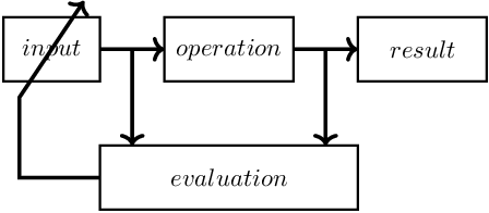
With negative feedback, the output of a system is compared to its intended output and if there is a difference between the two, the input signal into the system is adjusted in order to decrease the difference between the actual and the intended output. The “feedback” in “negative feedback” refers to adjusting the input of a system based on its output, while the “negative” refers to decreasing the difference between the actual and intended output.

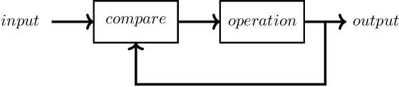
A block schematic representation of the principle of feedback is depicted in Figure 6.1. In this chapter, feedback is used on a system level for electronic circuits⁴⁴ , where the basic principle of Figure 6.1 is specified a bit more, resulting in the high level of abstraction representation given in Figure 6.2.

Feedback can be categorized into negative feedback and positive feedback. For negative feedback, the taken measure aims at counteracting some cause. Conversely, positive feedback enforces the cause. Later in this chapter, some more specific definitions are given.

6.2 Negative feedback

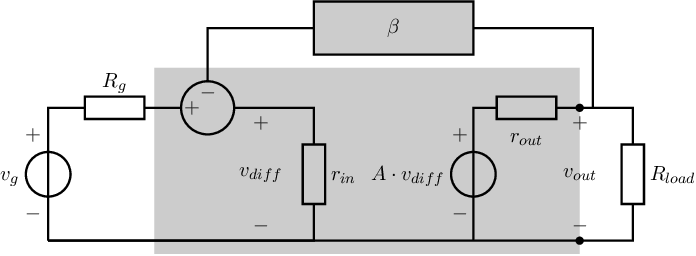
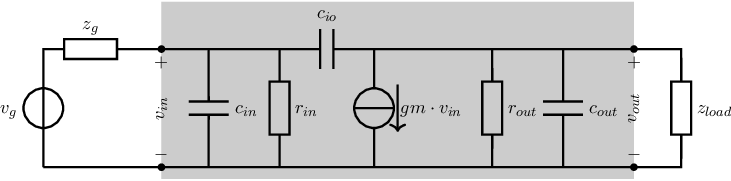
For an ideal voltage amplifier, the output voltage is independent of the load impedance. However, any real voltage amplifier has a non-zero output impedance, resulting in a non-zero dependency of the amplifier’s output voltage on the load impedance. Figure 6.3 shows an idealized voltage amplifier with output resistance $r_{out}$ , yielding for the loaded amplifier:

H = \frac{v_{out}}{v_{in}} = \frac{A \cdot R_{load}}{r_{out} + R_{load}} = \frac{A}{1 + \frac{r_{out}}{R_{load}}}

(6.1)

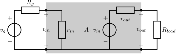
Equation (6.1) shows that if $R_{load}$ changes, so will the output voltage, which is usually an unwanted effect for a voltage amplifier. The root cause for this is the non-zero amplifier’s output resistance $r_{out}$ . Using feedback the effect of any load impedance on the output impedance will now be decreased. Note that this corresponds to decreasing the output impedance of the system composed of the amplifier and the feedback wrapped around it.

6.2.1 Full negative feedback: a first concept

This section presents a first concept for a voltage amplifier system using the amplifier in Figure 6.3, aiming at overall a minimum impact of $R_{load}$ on the overall voltage signal transfer. Note that this corresponds to a system with a small output resistance $r_{out} = v_{out} ∕ i_{out}$ . There are multiple ways to get the desired result:

increasing the voltage gain of the amplifier when detecting a too low output voltage (due to e.g. $R_{load}$ ).
using or creating an amplifier that has a negligibly small $R_{out}$ compared to $R_{load}$ .
making the driving voltage $v_{diff}$ for the amplifier dependent on both the signal source voltage $v_{g}$ and on the load-dependent output voltage $v_{out}$ in such a way that $v_{diff}$ increases as $v_{out}$ decreases and vice versa.

The first two options are in contradiction with the assumption on using the same amplifier as in Figure 6.3. For the third method — using feedback from the output to the input — one extra “component” must be used: a subtraction point⁴⁵ , leading to the systematic representation of Figure 6.4. In Figure 6.4 the actual input voltage of the amplifier $v_{diff}$ equals the difference between $v_{g}$ and $v_{out}$ :

v_{diff} = v_{g} - v_{out}

(6.2)

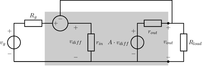
The voltage signal transfer of this circuit can easily be determined. Using the brute force method for the circuit in Figure 6.4, and assuming that the input impedance at each of the subtractor terminals is infinite, we may get:

\begin{array}{rcl} H & = \frac{v_{out}}{v_{g}} \\ v_{out} = A \cdot (v_{g} - v_{out}) \cdot \frac{R_{load}}{R_{out} + R_{load}} \\ v_{out} (1 + A \cdot \frac{R_{load}}{R_{out} + R_{load}}) = A \cdot v_{g} \cdot \frac{R_{load}}{R_{out} + R_{load}} \\ H & = \frac{A \frac{R_{load}}{R_{load} + R_{out}}}{1 + A \frac{R_{load}}{R_{load} + R_{out}}} & (6.3) \end{array}

From (6.3) it follows that for $A \cdot \frac{R_{load}}{R_{load} + R_{out}} > > 1$ the signal transfer function $H$ approaches to “only” 1, but that at the same time the $H$ is highly independent of variations in $R_{load}$ . This insensitivity nicely can be shown from the system’s output resistance $r_{out}^{'}$ . Calculating the output resistance as the quotient of open voltage and short circuit current (with a non-zero $v_{g}$ ):

\begin{array}{rcl} r_{out}^{'} & = & \frac{open voltage}{short - circuit current} \\ = & \frac{{v_{out} (v_{g}) |}_{R_{load} \to \infty}}{{i_{out} (v_{g}) |}_{R_{load} = 0 Ω}} \\ = & \frac{v_{g} \cdot \frac{A}{1 + A}}{\frac{v_{g}}{\frac{R_{out}}{A}}} \\ = & \frac{R_{out}}{1 + A} & (6.4) \end{array}

Alternatively, calculating the output resistance by forcing an output voltage or current (with $v_{g} = 0$ ):

\begin{array}{rcl} r_{out, amplifier}^{'} & = & {\frac{v_{out}}{i_{out}} |}_{v_{g} = 0} \\ = & \frac{v_{out}}{\frac{v_{out} \cdot (1 + A)}{R_{out}}} = \frac{R_{out}}{1 + A} & (6.5) \end{array}

From (6.4) and (6.5) it can directly be seen that the system’s output resistance is a factor $(1 + A)$ lower than the output resistance of the circuit without feedback. Also it follows that if the voltage gain $A$ is large, the output resistance is very small. Furthermore, it follows from (6.3) that the voltage gain of the original amplifier, $A$ , is also decreased by the factor $(1 + A)$ . This exchange between gain and improvement of some amplifier property in feedback systems is fundamental. It also implies that it is quite nice to use amplifiers that have very high gain to start with: other parameters can be optimized by sacrificing part of that gain.

6.2.2 Negative feedback: a generalised concept

Full negative feedback was introduced in §6.2.1. For full negative feedback, the entire output signal is subtracted from the actual input signal. However, we can also subtract just a part of the output signal from the input signal; this is the subject of this section.

Starting with the system in Figure 6.5, it is now assumed that the feedback is realised via an attenuating circuit with zero phase shift (for instance with a resistive divider or a capacitive divider, or whatever). The voltage gain of this circuit is denoted as $β$ , with here $0 \leq β \leq 1$ ⁴⁶.

The signal transfer of the circuit of Figure 6.5 can easily be derived. Note that with feedback typically separation of variables must be used to get a closed form expression.

\begin{array}{rcl} H = \frac{v_{out}}{v_{g}} \\ v_{out} = A \cdot v_{diff} \cdot \frac{R_{load}}{R_{out} + R_{load}} \\ v_{diff} = v_{g} - β \cdot v_{out} \\ v_{out} = A \cdot (v_{g} - β \cdot v_{out}) \cdot \frac{R_{load}}{R_{out} + R_{load}} \\ v_{out} (1 + A \cdot β \cdot \frac{R_{load}}{R_{out} + R_{load}}) = A \cdot v_{g} \cdot \frac{R_{load}}{R_{out} + R_{load}} \\ H = \frac{A \cdot \frac{R_{load}}{R_{out} + R_{load}}}{1 + A \cdot β \cdot \frac{R_{load}}{R_{out} + R_{load}}} & (6.6) \end{array}

Inspection of (6.6) reveals that for $Aβ \frac{R_{load}}{R_{load} + R_{out}} > > 1$ the equation can be approximated by

H = \frac{v_{out}}{v_{g}} \approx \frac{1}{β}

(6.7)

It follows that the signal transfer of the circuit in Figure 6.5 is largely insensitive to variations in $A$ , $R_{load}$ and $R_{out}$ . At the same time, the magnitude of $H$ is much lower than the open loop signal gain $A$ . A main advantage is that the closed loop signal transfer $H$ is determined by the attenuation factor $β$ . This attenuation factor $β$ can be made exact and linear using passive, linear components. Then using an ill defined but large $A$ yields a well defined closed loop gain $H \approx 1 ∕ β$ .

Finding e.g. the output resistance of the circuit including feedback, $R_{out}^{'}$ , is not very difficult. Using any proper analysis method yields $R_{out}^{'} = \frac{r_{out}}{1 + A \cdot β}$ . Note that the value of $R_{load}$ is not present in the output resistance of the circuit, since $R_{load}$ is external to the amplifier.

6.3 Negative feedback and amplifiers: some examples

Due to the quite sensitive — to everything, including temperature and processing spread — semiconductor devices required for circuits that contain components with power gain, obtaining well-defined amplifier properties (without feedback) is rather difficult. In this context, “well-defined” corresponds to properties with low sensitivity to variations in temperature, biasing conditions and more. Similarly “properties” correspond to things like a certain low or high output resistance or a large bandwidth. This section illustrates the effect of feedback on circuit properties, using a few examples.

6.3.1 Effect of negative feedback on bandwidth

An important parameter for every amplifier is the “-3 dB” frequency, or corner frequency. This frequency is usually determined by either an output load combined with the amplifier’s output resistance or by the (parasitic) load at some internal nodes in the amplifier, resulting in a frequency-dependent gain $A (jω)$ ; both items are addressed below.

Amplifier-limited bandwidth

Fundamentally, every internal node in an amplifier has resistive and capacitive loading. This is due to a few laws of physics and due to Maxwell with his nasty equations. As a result of this, e.g. the voltage gain of an amplifier cannot be frequency independent. Usually amplifiers are constructed in such a way that the frequency behavior mainly resembles first-order behavior⁴⁷ ; this type of amplifier is usually called “dominantly first-order” in its frequency behavior, for which then

\begin{array}{rcl} A (jω) & \approx & \frac{A_{0}}{1 + jω ∕ ω_{0}} \end{array}

Using this amplifier in a negative feedback configuration, as shown in Figure 6.6, without $Z_{load}$ , yields the following signal transfer for the circuit including feedback:

\begin{array}{rcl} H & = & \frac{A_{0}}{1 + A_{0} β} \cdot \frac{1}{1 + j \frac{ω}{ω_{0} (1 + A_{0} β)}} \end{array}

This relation shows that the -3dB frequency of the feedback system is increased by a factor $(1 + Aβ)$ with respect to the open loop situation, while the gain at low frequencies is decreased by the same factor. As usual for feedback configurations with negative feedback, an improvement in some property is paid for by a similar decrease in gain.

Load-limited bandwidth

The load impedance of an amplifier can typically be modelled as the series connection of a resistive load and a capacitive load while the output impedance of the circuit behaves resistively⁴⁸ . Then using negative feedback around the amplifier yields the circuit schematic in Figure 6.6:

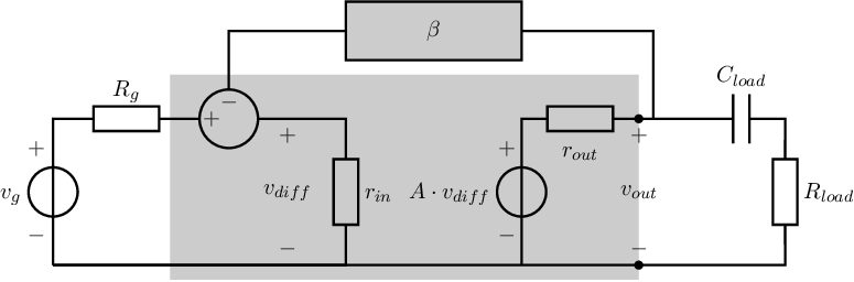
The voltage transfer of the circuit in Figure 6.6 can be determined using e.g. the brute force method as:

\begin{array}{rcl} H & = & \frac{v_{out}}{v_{g}} \\ v_{out} = \frac{Z_{load}}{Z_{load} + r_{out}} \cdot A \cdot v_{diff} \\ v_{diff} = v_{g} - β \cdot v_{out} \\ Z_{load} = R_{load} + \frac{1}{jω C_{load}} & (6.8) \end{array}

Now the hard part of the derivation is completed: only the (back)substitution must be done and possibly rewriting the result in a nice readable form may be required. Note that rewriting inherently does not change the equation, just its appearance or its usability.

\begin{array}{rcl} v_{out} = \frac{Z_{load}}{Z_{load} + r_{out}} \cdot A \cdot (v_{g} - β \cdot v_{out}) \\ v_{out} \cdot (1 + Aβ \frac{Z_{load}}{Z_{load} + r_{out}}) = A \cdot \frac{Z_{load}}{Z_{load} + r_{out}} v_{g} \\ H & = & \frac{A \cdot \frac{Z_{load}}{Z_{load} + r_{out}}}{1 + Aβ \frac{Z_{load}}{Z_{load} + r_{out}}} \end{array}

This signal transfer function corresponds to that of an amplifier with a first-order frequency dependent $A′ (jω) = A \cdot \frac{Z_{load}}{Z_{load} + r_{out}}$ using feedback factor $β$ . Again, the negative feedback decreases the voltage gain by a factor $(1 + A′β)$ which factor equals the factor at which the corner frequency is increased due to the negative feedback. Note that there is really no need to expand $Z_{load}$ unless an expression for e.g. the -3dB frequency must be derived, expressed in e.g. $C_{load}$ and $R_{load}$ .

6.3.2 Effect of negative feedback on interference, distortion and noise

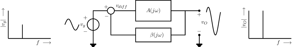
Interference is a phenomenon where signals from external sources or system parts couple into your circuit. Noise is generated in every circuit that dissipates energy due to plain physics. Distortion occurs in every system that includes non-linear components such as transistors. If interference, distortion or noise is present at the input of an amplifier, then there is nothing you can do to discriminate between the input signal and the noise, distortion or interference. However, if some unwanted signal is generated “somewhere in the circuit”, then there is a solution to suppress that. In this section, we start with the two circuits in the figure below, where noise, harmonic contents or interference is represented by the source $v_{st}$ .

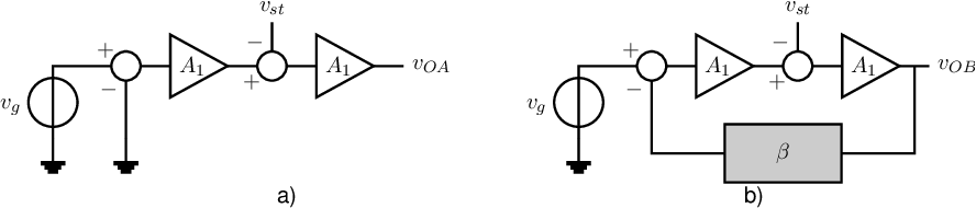
For fair comparison of the effect of feedback, let’s assume the two configurations below. The leftmost amplifier is without feedback where the amplifier on the right hand side uses negative feedback.

It may be illustrative to start at two extreme cases:

Injecting noise, distortion components or interference at the very output of the amplifier in the system, corresponding to $A_{2} = A_{4} = 1$ .

The output voltage of the two circuits is then:
$\begin{array}{rcl} v_{OA} & = & A_{1} \cdot v_{g} + v_{st} \\ v_{OB} & = & \frac{A_{3}}{1 + β A_{3}} \cdot v_{g} + \frac{1}{1 + β A_{3}} \cdot v_{st} \end{array}$
To ensure identical overall signal gain, the gain factors $A_{1}$ and $A_{3}$ are related as $A_{1} = \frac{A_{3}}{1 + β A_{3}}$ which reveals that any disturbance injected at the output of a system are suppressed by a factor $1 + β A_{3}$ or $A_{3} ∕ A_{1}$ which equals the reduction in gain due to using feedback.
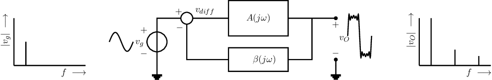
Injecting noise, interference or distortion components at the input of the amplifiers, for which $A_{1} = A_{3} = 1$ leading to the following expressions for the output voltage of the circuits:
$\begin{array}{rcl} v_{OA} & = & A_{2} \cdot v_{g} + A_{2} \cdot v_{st} \\ v_{OB} & = & \frac{A_{4}}{1 + β \cdot A_{4}} \cdot v_{g} + \frac{A_{4}}{1 + β \cdot A_{4}} \cdot v_{st} \end{array}$
To ensure identical overall signal gain in the systems with and without feedback, the gain factors $A_{2}$ and $A_{4}$ are related as $A_{2} = \frac{A_{4}}{1 + β A_{4}}$ . From this it can be concluded that disturbances injected at the input of the amplifier are not suppressed by loop gain.

These findings can be generalized: disturbances injected somewhere in the systems, dimensioned to deliver identical signal gain, are suppressed by the earlier reported factor $A_{3} ∕ A_{1}$ . Again, suppression of any disturbances injected somewhere in a feedback system is at the cost of overall signal gain of a system.

6.4 Stability

The previous sections of this chapter, showed that negative feedback results in less sensitive — to everything — amplifiers. Negative feedback is actually coupling (a part of) the output signal, in anti-phase, to the input. This anti-phase feedback is usually obtained by subtracting an in-phase signal from the input signal; the subtraction hence generates the required inversion.

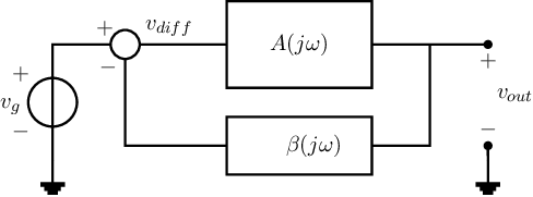
Up till now, it was assumed that the amplifiers used in the feedback systems were frequency independent. However, in reality, the forward gain $A$ and the feedback factor $β$ may be frequency dependent, written as $A (jω)$ and $β (jω)$ . Figure 6.7 represents the general schematic of a system with negative feedback. The signal transfer is

\frac{v_{out}}{v_{g}} = \frac{A (jω)}{1 + A (jω) β (jω)}

(6.9)

Due to their frequency dependency, the both $A (jω)$ and $β (jω)$ in general have non-zero frequency dependent phase shifts. In this case there may be an angular frequency $ω_{1}$ for which the phase shift of $A (j ω_{1})$ added to the phase shift of $β (j ω_{1})$ equals $- π$ :

\arg (A (j ω_{1}) β (j ω_{1})) = - π

(6.10)

For this specific angular frequency the (probably intended) negative feedback becomes actually positive feedback: the fed back signal experiences an inversion (due to the subtraction) and has a phase shift of $- π$ , resulting in a net phase shift of 0. In that case the original negative feedback turns into positive feedback. Systems with positive feedback can be stable, can be oscillating or or can be unstable; the actual type of behavior depends on the magnitude of the loop gain of the system, $A (ω) β (ω)$ as will be explained in this section. Also the degree of stability, stability criteria and possible stability representations are discussed.

6.4.1 Rough classification of systems with feedback

The loop gain $A (jω) β (jω)$ of a system with feedback determines the behavior of that system. This loop gain partly determines (among others) the magnitude of the input signal of the amplifier:

\begin{array}{rcl} v_{in - amplifier} & = & v_{G} - β \cdot v_{OUT} \\ = & v_{G} - β \cdot \frac{A (jω)}{1 + A (jω) β (jω)} \cdot v_{G} \\ = & \frac{v_{G}}{1 + A (jω) β (jω)} & (6.11) \end{array}

Negative feedback may turn into positive feedback if the phase shift of the loop gain $A (jω) β (jω)$ is an odd integer times $π$ . In this case $\arg (A (jω) β (jω)) = π \pm 2 nπ$ and hence the (real) value of $A (jω) β (jω) < 0$ . Inspection of (6.11) shows that the denominator can become “0” or even negative for negative real valued $A (jω) β (jω)$ .

If the denominator $1 + A (jω) β (jω) = 0$ at a certain frequency $ω_{0}$ , then every signal at $ω_{0}$ is amplified $\infty$ times. In that case, zero input signal may result in a non-zero output signal at this specific $ω_{0}$ . The result is then a circuit that generates a sinusoidal signal, all by itself, at a frequency $ω_{0}$ for which $1 + A (ω_{0}) β (ω_{0}) = 0$ . These so-called harmonic oscillators are discussed and analyzed in chapters 9 and 10.

If $(1 + A (jω) β (jω))$ is negative real at one frequency, then the system is unstable: it switches from one state to another depending on the input signal. The circuit behavior then is very non-linear, and hence for this region linear analysis methods and impedances cannot be used⁴⁹ . Switching circuits are useful in digital systems, in analog-to-digital converters and in relaxation oscillators. None of these is discussed in detail in this book.

Concluding, we can identify 4 situations for systems with negative feedback:

\begin{array}{rcl} A (jω) β (jω) |_{ω = ω_{0}} = - 1 & \to & oscillation for ω = ω_{0}, \\ harmonic oscillation at ω_{0}, chapters 9 and 10 \\ A (jω) β (jω) |_{ω = ω_{0}} < - 1 & \to & switching behavior, \\ positive feedback, not discussed in detail \\ Re (A (jω) β (jω)) |_{\forall ω} > 0 & \to & stable behavior, negative feedback \\ Re (A (jω) β (jω)) |_{ω = ω_{0}} < 0 & \to & stable behavior, positive feedback \\ or switching behavior, not discussed \\ or harmonic oscillation, chapters 9 and 10 \end{array}

6.4.2 Stability of systems with negative feedback

In this chapter, only stable systems with feedback are analyzed; harmonic oscillators are addressed in chapters 9 and 10 while hard-switching systems are not addressed in this book. As stated in §6.4.1, a system’s stability depends on the denominator of the signal transfer function of the system, $(1 + A (jω) β (jω))$ .

In 1932, Harry Nyquist presented an analysis of stability for systems with negative feedback. His mathematical analysis was based on Cauchy’s principle of argument published in the mid 1800’s.

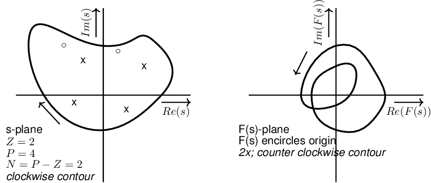
Cauchy’s principle of argument Let $F (s)$ be an analytic function in a closed region of the complex plane $s$ except at a finite number of points (namely, the poles of $F (s)$ ). It is also assumed that $F (s)$ is analytic at every point on the contour. Then, as $s$ travels around the contour in the $s$ -plane in the clockwise direction, the function $F (s)$ encircles the origin in the $Re (F (s)), Im (F (s))$ -plane in the same direction $N$ times, with $N$ given by $N = Z - P$ where $Z$ and $P$ stand for the number of zeros and poles (including their multiplicities) of the function $F (s)$ inside the contour.

The left-hand side figure below shows an example having 4 poles (indicated by a ” $x$ ”) and 2 zeros (indicated by a ” $\circ$ ”), all encircled by an arbitrary closed contour. The corresponding $F (s)$ -contour encircles the origin $N = 2 - 4 = - 2$ times in the same direction as the $s$ -contour. For this specific example, the $s$ -contour is clockwise and hence the $F (s)$ contour is counter clockwise, encircling the origin twice. Note that for another contour in the $s$ -plane the corresponding $F (s)$ -contour is different.

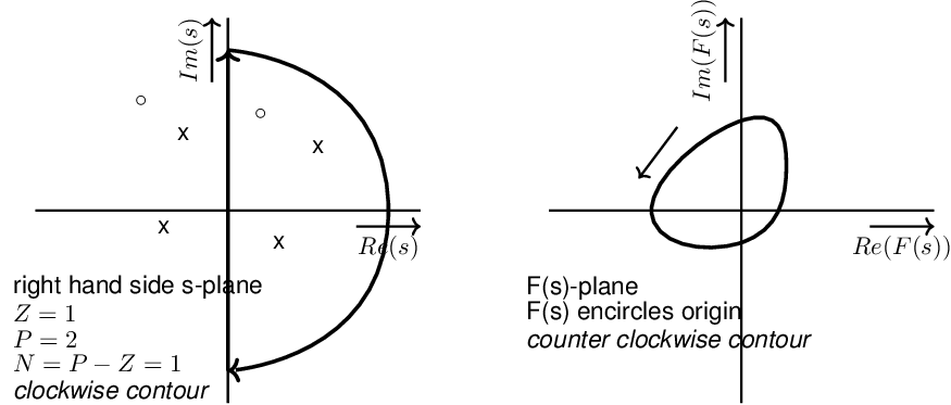
Illustration of Cauchy’s argument principle

Nyquist used (a variant of) Cauchy’s principle of argument using a specific path for $s$ , where he assumed for $s$ the (complex) frequency parameter used in Laplace analyses, $s = σ + jω$ . This $s$ has quite a lot of similarities to the $jω$ operator used in the regular frequency domain analyses - digging into Laplace is however out of scope for this book - all you need to know right now is that a term in a transfer function $H (s) = \frac{1}{s + a}$ has a pole at $s = - a$ and corresponds to an impulse response $h (t) = e^{- a \cdot t}$ . This impulse response shows that any pole that has a real positive part, $Re (- a) = σ > 0$ , is unstable. In mathematical terminology, right-half-plane (RHP) poles in the $s$ -plane correspond to unstable responses.

For this reason, Nyquist used a (clockwise) loop in the $s$ -plane that spans the total RHP: his clockwise closed loop starts at $s = 0$ and from there the radian frequencies increases from $ω = 0$ to $ω \to \infty$ . After that, the $s$ -path continues in the clockwise direction via a half-circle $| s | \to \infty$ back to $ω \to - \infty$ . The last part is sweeping the radian frequency from $ω \to - \infty$ back to $ω = 0$ . Wherever there is a pole on the imaginary axis in the $s$ -plane, an infinitesimal detour is made around this pole in such a way that these poles are excluded from the contour.

Nyquist used the denominator of a feedback system as $F (jω)$ : $F (s) = 1 + A (jω) β (jω)$ , now written as $F (s) = 1 + A (s) β (s)$ . Another essential step in Nyquist’s work is to note that zeros of $F (s) = 1 + A (s) β (s)$ are equal to poles of the overall (closed loop) transfer function and that the poles of $F (s)$ are the poles of the open loop response of the system.

Nyquist’s use of Cauchy’s principle of argument

Using all this, conclusions on the stability of feedback systems can be drawn. The most widely applied one in electronics assumes (usually implicitly) that the open-loop system (without feedback) is stable. In that case the open loop system has no RHP poles; in Cauchy-terms this corresponds to $P = 0$ for the contour used by Nyquist. A closed loop response that also does not have RHP-poles is then stable, and this translates into the demand that $F (s)$ does not have RHP zeros, or Z=0. Then the overall requirement for stability is $N = Z - P = 0$ and the contour of $F (s)$ is hence not allowed to encircle the origin of the $F (s)$ -plane.

Finally, Nyquist did not plot $F (s) = 1 + A (s) β (s)$ but omitted the “1” leading to $F (s) = A (s) β (s)$ and consequently leading to N-times encircling the “-1” instead of encircling the origin in the $F (s)$ -plane.

From the analysis of Harry Nyquist, a number of interesting conclusions concerning stability have been drawn. To estimate the (degree of) stability of a system with feedback, Nyquist introduced a polar figure (also known as the Nyquist-plot) in which the complex loop gain $A (jω) β (jω)$ is plotted as a function of (angular) frequency $ω$ . As shown in the grey region above, Nyquist derived that:

If the contour of

A (jω) β (jω)

in the polar figure does not circle the point

{- 1, 0}

in the clockwise direction with

ω

increasing from

- \infty

\infty

, then the corresponding system (with feedback) is stable. If this

{- 1, 0}

-point is encircled in the clockwise direction with increasing

ω

, then the system is unstable.

Note that this all-determining “-1” point in the complex plane is nothing more or less than the value at which the denominator in any closed loop transfer function, $(1 + A (jω) β (jω)$ ), is zero.

6.4.3 Stable and unstable: now what?

The stability of a system depends on $A (jω) β (jω)$ . For stable systems, the polar plot of $A (jω) β (jω)$ does not encircle the ${- 1, 0}$ point in a clockwise direction with increasing $ω$ . For unstable systems, the ${- 1, 0}$ point is encircled in the clockwise direction.

Stable systems can display unwanted behavior such as overshoot, ringing or undershoot, but after sufficient time, the system’s output signal settles to a (complex) multiple of its input signal. A number of examples are given in §6.4.4. For an unstable system, the output voltage will continue to grow in time to $\pm \infty$ , until it hits some physical or implementation limit.

Both linear and non-linear networks can be analyzed using element equations in time domain. Only linear(-ish) networks can be analyzed in the frequency domain, using impedances, due to the linear transformation underlying the derivation of impedances from element equations. It then directly follows that

Stable linear systems can be analyzed in both the time and frequency domains.
If a stable system’s output signal hits some limit (e.g. the supply voltage) the system effectively is non-linear, see Figure 6.9. In this case, or if the system by itself is very nonlinear, analyses in the frequency domain may not be appropriate⁵⁰ .
An unstable system cannot be analyzed in the frequency domain: the circuit will operate heavily nonlinearly and the linear transformations underlying everything in the frequency domain cannot be used. The only correct way to analyze unstable circuits is doing analyses in the time domain.

6.4.4 Stability of systems with feedback: examples

As stated in §6.4.2, the stability of a system depends on the trajectory of $A (jω) β (jω)$ in the complex plane (the Nyquist plot) and whether the point ${- 1, 0}$ is encircled in the clockwise direction with increasing $ω$ . This section gives a number of examples.

First-order (low-pass) systems are probably the simplest frequency-dependent systems. Assuming a frequency-independent $β$ , and a first-order low-pass $A (jω)$ :

\begin{array}{rcl} H (jω) & = & \frac{A (jω)}{1 + A (jω) β (jω)} \\ = & \frac{A_{0}}{1 + A_{0} β} \cdot \frac{1}{1 + j \frac{ω}{ω_{0} \cdot (1 + A_{0} β)}} \\ A (jω) β (jω) & = & \frac{A_{0} β}{1 + jω ∕ ω_{0}} & (6.12) \end{array}

From this it follows immediately that $A (jω) β (jω)$ can never be equal to -1: the real part of $A (jω) β (jω)$ is always larger than or equal to zero. Systems for which $A (jω) β (jω)$ is first-order low-pass are hence unconditionally stable.

The Nyquist plots for a first order low pass characteristics visualize this. Creating a Nyquist plot can be done analytically for first-order systems, yielding a half-circle for $0 \leq ω \leq \infty$ and a half-circle for negative frequencies $- \infty \leq ω \leq 0$ . These are drawn in blue and grey respectively in Figure 6.10. The left hand side Nyquist plot in in Figure 6.10 is for $A_{0} = 10$ and $β = 1$ while the right hand side version assumes $A_{0} = 10$ and $β = 0.5$ . In both Nyquist plots, $ω \to \infty$ is indicated (located at the origin of the plots) and the direction of increasing (radian) frequency is indicated. Lastly, the $(- 1, 0)$ point is indicated.

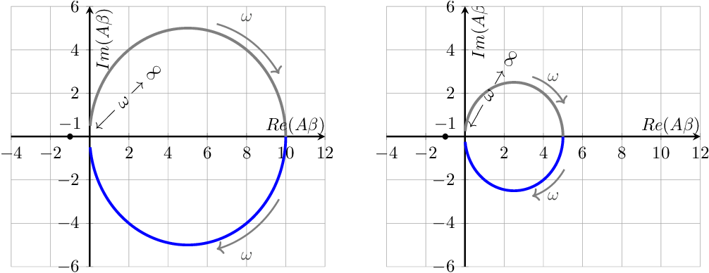
Note that for any Nyquist plot, the contour for negative and positive frequencies are identical, except for mirroring in the real axis. In general Nyquist plots must be made numerically⁵¹ and stability is usually derived from the Nyquist plot.

It is not possible to get the signal transfer function of a system from its

A (jω) β (jω)

: only the (degree of) stability can be derived from it. For example for a first-order low-pass

A (jω) β (jω)

, where the first-order characteristic is either in

A (jω)

β (jω)

\begin{array}{rcl} A (jω) β (jω) = \frac{A_{0} β_{0}}{1 + jω ∕ ω_{0}} \\ 1: & A (jω) = \frac{A_{0}}{1 + jω ∕ ω_{0}} \to H (jω) = \frac{A_{0}}{1 + A_{0} β} \cdot \frac{1}{1 + j \frac{ω}{ω_{0} \cdot (1 + A_{0} β)}} \\ 2: & β (jω) = \frac{β_{0}}{1 + jω ∕ ω_{0}} \to H (jω) = \frac{A_{0}}{1 + A_{0} β} \cdot \frac{1 + j \frac{ω}{ω_{0}}}{1 + j \frac{ω}{ω_{0} \cdot (1 + A_{0} β)}} \end{array}

The first signal transfer is clearly a first-order low-pass, while the second is a combination of high-pass and low-pass characteristics, for the same

A (jω) β (jω)

Second-order (low-pass) systems are a bit more complex than first-order systems. For a second-order low-pass $A (jω)$ with a real feedback factor $β$ :

\begin{array}{rcl} A (jω) β (jω) & = & \frac{A_{0} β}{1 + j \frac{ω}{Q ω_{0}} + {(j \frac{ω}{ω_{0}})}^{2}} & (6.13) \end{array}

Deriving a readable expression for the shape of the Nyquist plot, and plotting it requires quite some work. As alternative, a few distinct points on the Nyquist contour can readily be calculated and can be used a guide to sketch the full Nyquist plot. Most easy is to pick a few (convenient) positive $ω$ -s:

$ω = 0$
$ω = ω_{0}$
$ω \to \infty$

The complete Nyquist contour must be drawn for $- \infty \leq ω \leq + \infty$ . However, noting that the contour for negative frequencies is the mirrored (in the real axis) version of the contour for positive frequencies, deriving the full contour from the contour for positive frequencies is quite straight forward. From the specific positive frequencies mentioned above, we get a phase shift and magnitude of $A (jω) β (jω)$ equal to

0 $^{\circ}$ respectively $| A (jω) β (jω) | = A_{0} β$ for $ω = 0$
-90 $^{\circ}$ respectively $| A (jω) β (jω) | = Q \cdot A_{0} β$ for $ω = ω_{0}$
-180 $^{\circ}$ respectively $| A (jω) β (jω) | = 0$ for $ω \to \infty$ .

Because the phase of $A (jω) β (jω) \geq - 18 0^{\circ}$ , it can be concluded that the Nyquist contour of a second-order system cannot encircle the (-1,0) point. Not in the clockwise direction nor in the anticlockwise direction. It cannot. Hence a second-order system is unconditionally stable.

It can however be derived that the Nyquist contour may be very close to the (-1,0) point in the Nyquist plot, depending on $A_{0}$ , $Q$ and $β$ when assuming (6.13). If the Nyquist contour gets close to the $(- 1, 0)$ -point, then the denominator $(1 + A (jω) β (jω))$ — that is used for about everything in feedback systems — becomes very small and the signal transfer function $H (jω)$ may get large. This $H (jω)$ then can show significant peaking, or a desired low output impedance can be very high around the corresponding frequency.

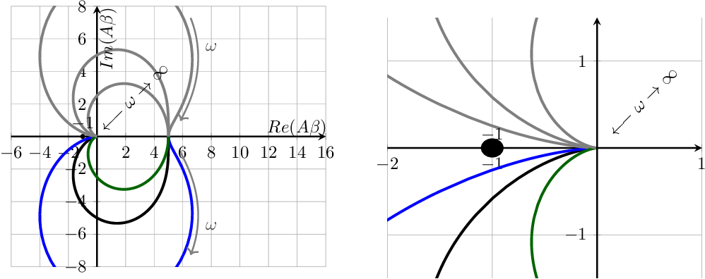
An illustration is given in the next two figures. The plot on the left hand side of Figure 6.11 shows three Nyquist contours, for three different values for Q with $A (jω) β (jω)$ according to (6.13). The right-hand side plot in Figure 6.11 zooms in on the area around the –1 point: none of the polar plots encircles or crosses the –1 point although there is just a small clearance between the curve and the –1 point.

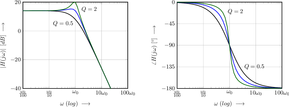
The stability of a system can be seen very clearly in a Nyquist plot (further on we also introduce the degree of stability), but the signal transfer of the system cannot be obtained from this plot. The signal transfer $H (jω)$ corresponding to the $A (ω) β (ω)$ curves in Figure 6.11 and assuming a real valued $β$ are given in Figure 6.12.

Higher-order (low-pass) systems are again a bit more complex than second-order systems, hence they can have more phase shift. In general, an $n^{th}$ -order low-pass system can have a phase shift of $n \cdot - 9 0^{\circ}$ for positive frequencies. From this it follows that all systems of third or higher order might have sufficient phase shift to encircle the –1 point in the Nyquist plot in the clockwise direction: they may get unstable⁵² .

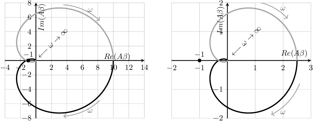
In Figure 6.13, the Nyquist plots of two third-order low-pass systems are shown. Both have a maximum phase shift of $n \cdot - 9 0^{\circ} = - 27 0^{\circ}$ for $0 \leq ω \leq + \infty$ . For one system $A (jω) β > 1$ for the $ω$ at which the phase shift equals $- 18 0^{\circ}$ resulting in clockwise encircling the –1 point. This corresponds to an unstable system. The other has a much smaller loop gain (for instance due to a smaller $β$ ) and there the corresponding Nyquist curve does not encircle the –1 point: this system is stable.

6.4.5 Phase and gain margin

The Nyquist plots show whether a feedback system is stable or unstable. As you probably already figured out: this is a yes/no answer, the system is stable or not. In this context, an unstable system has a diverging output signal (magnitude) for any non-zero input signal; a stable system has a bounded output signal for a bounded input signal. For normal systems, the stability requirement is much more strict than “just stable”: usually sufficient flat frequency response or sufficiently fast settling behavior after the occurrence of an input signal step is required. This can all be nicely described by stability margins:

\begin{array}{rcl} The stability margin corresponds to the distance (margin) \\ between the A (jω) β (jω) contour and –1 \end{array}

The definition above can be redefined in two ways, since the loop gain $Aβ$ is a complex curve (i.e. a curve in the complex plane).

One stability margin corresponds to the ratio between $| A (jω) β (jω) |$ and $| - 1 |$ for the (angular) frequency where $\arg (A (jω) β (jω)) = - 18 0^{\circ}$ . This ratio corresponds to the extra gain required for the system to make the $| A (jω) β (jω) |$ actually cross the –1 point.
This type of margin is denoted as gain margin.
The other stability margin is the angular distance between $\arg (A (jω) β (jω))$ and $\arg (- 1)$ for the frequency where $| A (jω) β (jω) | = | - 1 |$ . This angular distance is the extra phase shift required to make the $| A (jω) β (jω) |$ cross the –1 point.
This type of margin is denoted as phase margin.

If both the gain margin and the phase margin of a system are small, then there is only little room for spread in any parameter of $A (jω) β (jω)$ before the system becomes unstable; such a system is usually called marginally stable.

Phase margin is derived for the

ω

that satisfies

| A (jω) β (jω) | = 1

and represents the difference between

\arg (A (jω) β (jω))

and

- π

. The phase margin is positive if the system is stable.

Gain margin is defined for the

ω

that satisfies

\arg [A (jω) β (jω)] = - π

and represents the ratio between 1 and

| A (jω) β (jω) |

(hence equals

1 ∕ | A (jω) β (jω) |

). If the gain margin is larger than 1 or positive in [dB], then the system is stable.

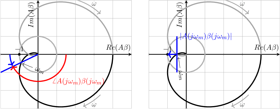
The left hand side Nyquist plot in Figure 6.14 illustrates the phase margin concept. For this, the (angular) frequency at which $| A (jω) β (jω) | = 1$ is denoted as $ω_{m}$ and is at the intersect of a unit circle (gray) and the Nyquist contour (black). The corresponding phase shift $∠A (j ω_{m}) β (j ω_{m})$ is marked by the red arrow. The phase margin is the angular difference between the (negative) real axis and the (here blue) line from the origin through the forenamed intersect. This phase margin is depicted by the blue arrow; in this example the phase margin is about $2 5^{\circ}$ .

The right hand side Nyquist plot in Figure 6.14 illustrates the gain margin concept. The (angular) frequency at which $∠A (jω) β (jω) = - 18 0^{\circ}$ is denoted as $ω_{m}$ . The gain margin is the extra gain that would be required to have the contour cross the –1-point: $1 ∕ | A (j ω_{m}) β (j ω_{m}) | = 1$ , illustrated by the blue arrow.

Examples of

The degree of stability and both of the introduced measures of stability may not mean much to you right now, so below some examples are presented on stability margins and on their impact for a few stable feedback systems. This is done by giving the step response and the polar figure of the systems. Also some corresponding Bode plots are shown.

This example uses 2 systems: a first-order and a second order system. As derived earlier, both systems are fundamentally stable, although the $A (jω) β (jω)$ curve of the second-order system may get very close to the –1 point in a Nyquist plot. The systems have an open loop gain of:

\begin{array}{rcl} A_{1} (jω) & = & \frac{A_{0}}{1 + j \frac{ω}{ω_{0}}} \\ A_{2} (jω) & = & \frac{A_{0}}{1 + j \frac{ω}{Q \cdot ω_{0}} + {(j \frac{ω}{ω_{0}})}^{2}} \end{array}

For the first-order system we have the following closed loop gain (with a passive, non-phase-shifting, feedback factor $β$ ):

\begin{array}{rcl} H_{1} (jω) & = & \frac{A_{1} (jω)}{1 + A_{1} (jω) \cdot β} = \frac{A_{0}}{1 + A_{0} β + j \frac{ω}{ω_{0}}} \\ = & \frac{A_{0}}{1 + A_{0} β} \cdot \frac{1}{1 + j \frac{ω}{ω_{0} \cdot (1 + A_{0} β)}} \end{array}

This equation shows that with negative feedback, the DC gain becomes smaller while the bandwidth increases:

\begin{array}{rcl} ω_{0, 1}' & = & ω_{0} \cdot (1 + A_{0} β) and A_{0, 1}' = \frac{A_{0}}{1 + A_{0} β} \end{array}

For second-order systems, also assuming a passive feedback system without phase shift, something similar follows:

\begin{array}{rcl} H_{2} (jω) & = & \frac{A_{2} (jω)}{1 + A_{2} (jω) \cdot β} = \frac{A_{0}}{1 + A_{0} β + j \frac{ω}{Q \cdot ω_{0}} + {(j \frac{ω}{ω_{0}})}^{2}} \\ = & \frac{A_{0}}{1 + A_{0} β} \cdot \frac{1}{1 + j \frac{ω}{Q \cdot ω_{0} \cdot (1 + A_{0} β)} + {(j \frac{ω}{ω_{0} \cdot \sqrt{1 + A_{0} β}})}^{2}} \end{array}

Similar as for the first-order system, with negative feedback the DC gain decreases and the bandwidth increases. Furthermore, the quality factor Q is now dependent on $β$ :

\begin{array}{rcl} ω_{0, 2}' & = & ω_{0} \cdot \sqrt{1 + A_{0} β} \\ A_{0, 2}' & = & \frac{A_{0}}{1 + A_{0} β} \\ Q′ & = & Q \cdot \sqrt{1 + A_{0} β} \end{array}

The Nyquist plots for the first-order system and for the second=order system are presented in the figure below. For both $A_{0} = 10$ is chosen while for the second order system, $Q = 1$ is assumed. The Nyquist contours for both systems without feedback (or equivalently for $β = 0$ ) is presented on the left hand side graph. Note that the Nyquist “curves” collapse to the origin due to $β = 0$ . Note that in all figures, the unit circle is shown and — whenever applicable — also the phase shift $∠A (jω) β$ for $| A (jω) β | = 1$ is shown.

left: Nyquist plots for the first order and second order systems without feedback.

center: Nyquist plots assuming

β = 0.15

right: Nyquist plots assuming

β = 0.8

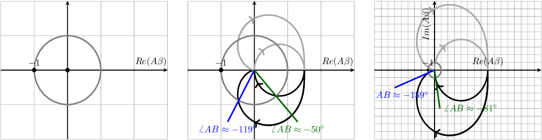
The center Nyquist plots assumes $β = 0.15$ . These plots show that the phase margin of the first order system is about $13 0^{\circ}$ and that the phase margin of the second order system is roughly $6 1^{\circ}$ . For both, the gain margin is $\infty$ .

The right hand side figure show the Nyquist plots for $β = 0.8$ . Here, the phase margins for the systems are approximately $9 9^{\circ}$ and $2 1^{\circ}$ . Note that this plot is on a different scale as compared to the previous two to be able to show the full Nyquist contours. Also here, the gain margin is $\infty$ .

A Bode plot can also be used to show the degree of stability of a system when plotting the loop gain of a system. This is worked out in section 6.5. The Bode plots below represent the closed loop transfer $H (jω)$ of the first-order and second-order systems that were used for the Nyquist plots above.

Bode plots for the first order systems for

β = 0

β = 0.15

and

β = 0.8

;

A_{0} = 10

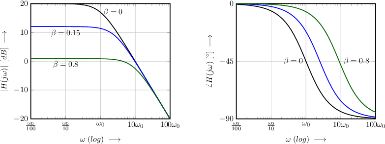
First order systems with passive, zero phase shifting feedback networks are stable, which follows from their Nyquist plots. With increasing $β$ , the signal transfer $H (jω)$ decreases at low frequencies, the bandwidth increases and the high frequency behavior is (almost) unchanged.

Second order systems as treated in the Nyquist plots above — $A_{0} = 10$ , open loop $Q = 1$ and with zero phase shifting feedback — are also always stable. As shown in the Nyquist plots, with increasing $β$ the phase margin decreases. In the Bode plot of the signal transfer function $H (jω)$ this decreased phase margin results in peaking around the corner frequency.

Bode plots for the second order systems for

β = 0

β = 0.15

and

β = 0.8

;

A_{0} = 10

and for the system without feedback

Q = 1

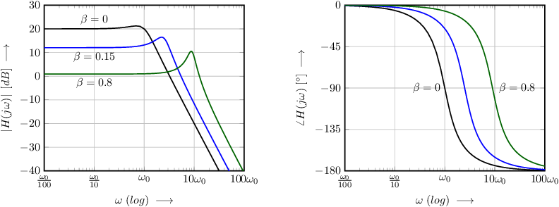
All systems treated sofar are stable: the Nyquist contour does not encircle the –1 point (at all, including in the clockwise direction). Note that for unstable systems, it is impossible to make a Bode diagram of the signal transfer function, since the system is not operating linearly while the Bode plot implicitly assumes a linear transfer!

The step responses for the three situations clearly show the effects of the phase margins. Step responses for the first-order and second-order systems discussed throughout this example are shown in the figure below. For the three plots, the input step-size was kept constant.

left: step responses for the two systems without feedback.

center: step responses for the two systems with a small negative feedback.

right: step responses for the two systems with a larger negative feedback

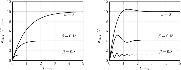
From the above graphs, it is evident that reduced phase margins (and similarly reduced gain margins) result in more ringing: the response is less stable. However, as long as the system as a whole is stable, then the ringing will eventually die out and the system is considered to be stable. If the point –1 is crossed by the $A (jω) β (jω)$ contour, then the response is a stable harmonic signal, which is used later in this book for creating harmonic oscillators. For systems that encircle –1 in the clockwise direction, the response to anything will continue to grow over time; these systems are really unstable in any aspect.

6.5 The Bode plot as tool for presentation

The polar diagram of $A (jω) β (jω)$ gives a lot of insight in the stability properties of feedback systems, but the interpretation of polar curves with frequency as implicit parameter may be difficult. Furthermore, the dynamic range of a system (the difference between the smallest and largest value of the transfer) may be very large causing important details to be hidden/not observable. An example of this is in Figure 6.11, where you have to zoom in quite far to really say something about the stability around the –1 point. This is the main reason for using a logarithmic Bode plot when designing or evaluating feedback systems.

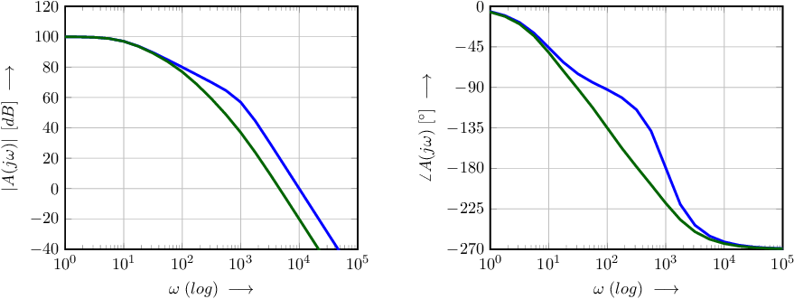
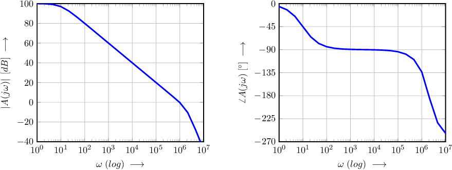
Using a Bode plot — instead of the Nyquist plot — to evaluate stability issues, the loop gain $A (jω) β (jω)$ now must be plotted instead of the (closed loop) transfer function. In this section, an amplifier with a third-order low-pass characteristic as an example. The general transfer function of such a circuit is:

\begin{array}{rcl} A (jω) & = & \frac{A_{0}}{(1 + j \frac{ω}{ω_{1}}) (1 + j \frac{ω}{ω_{2}}) (1 + j \frac{ω}{ω_{3}})} or \\ = & \frac{A_{0}}{(1 + j \frac{ω}{ω_{1}}) (1 + j \frac{ω}{Q ω_{0}} + {(j \frac{ω}{ω_{0}})}^{2})} \end{array}

The overall transfer function is decomposed in three (real) first-order transfer functions in the first notation. The second notation is valid if the original transfer function cannot be decomposed into three real first-order transfer functions: a decomposition into one first-order and one second-order transfer function can be done. Both are plotted in Figure 6.15.

The (degree of) stability can be estimated from the Nyquist plot of the loop gain $A (jω) β (jω)$ . This loop gain may not enclose the –1 point in the clockwise direction (with increasing $ω$ ) for a stable system. The phase margin and gain margin show the degree of stability.

The Bode plot can also be used to determine phase and gain margin. To do so, the loop gain $A (jω) β (jω)$ must be plotted, after which the phase margin and gain margin can be estimated applying the definition of these two margins. This will be clarified using a few examples.

Stability with a real valued $β$

For Figure 6.16, a feedback factor to 0.01 (-40dB) is applied to both systems in Figure 6.15. The Bode plot of the loop gain $A (jω) β (jω)$ is then simply 40 dB lower than the open loop curve $A (jω)$ and the phase characteristic is identical to that of $A (jω)$ . Note that this yields a closed loop signal transfer function that ideally equals $H \approx 1 ∕ β = 100$ .

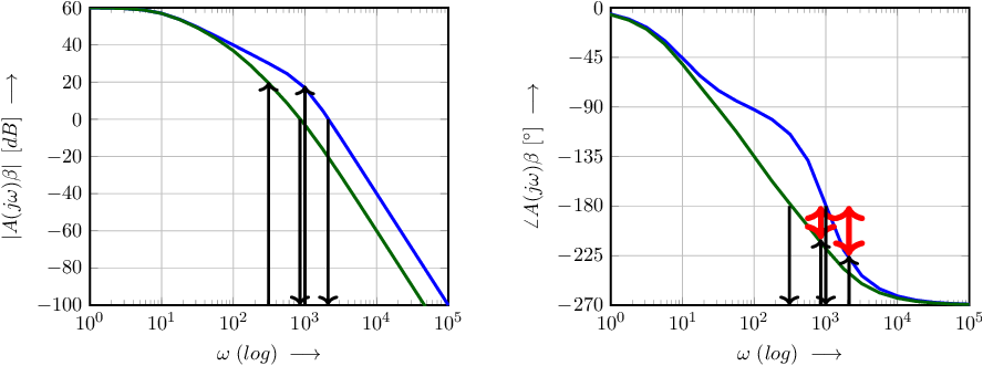
The critical point for stability is –1 point. In Bode-terms, this –1 point corresponds to 0 dB magnitude and -180 $^{\circ}$ phase shift.

The gain margin can be estimated by getting the (radian) frequency at which $∠Aβ = - 18 0^{\circ}$ in the phase plot and getting the corresponding gain at that frequency in the magnitude plot. This is indicated by the downward arrows in the phase plot and the upward arrows in the magnitude plot. In Figure 6.16 the gain margins are negative — about $- 3 0^{\circ}$ and $- 4 5^{\circ}$ — and both systems are unstable.

Similarly, the phase margin can be estimated by getting the (radian) frequencies at which $| Aβ | = 1$ from the magnitude part of the Bode plot and getting the corresponding phase shift from the phase plot. This is represented by the downward arrows in the magnitude plot and the upward arrows in the phase plot. It appears that also the phase margins are negative — about $- 20 dB$ nd $- 18 dB$ — another indication for unstable systems.

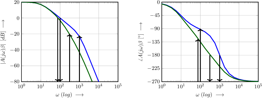
The systems in Figure 6.16 are unstable. Decreasing the (zero phase shifting) feedback factor yields a more stable (less unstable) system. Figure 6.17 shows the above systems, but now with a smaller feedback factor: $β = 0.0001 ≜ - 80 dB$ , yielding ideally a signal gain factor of about 80dB. The Bode plot of the loop gains show that the gain margins are now $20 dB$ and $22 dB$ , and that the phase margins are $5 0^{\circ}$ and $9 0^{\circ}$ : both systems are stable using this $β$ .

6.6 Feedback and dominant first-order behavior

To create a stable system with feedback, a sufficient phase margin and gain margin must be ensured. As shown previously, estimating these margins requires calculating $A (jω)$ and $β (jω)$ for every feedback system, and checking whether it is sufficiently stable. Obviously, this poses a problem, mainly because time is scarce and we prefer playing games instead of calculating Bode plots or Nyquist plots.

The design process of a (stable) amplifier with feedback can be simplified using idiot-proof amplifiers. Idiot-proof amplifier are designed in such a way that they are stable with any real valued attenuating $β$ . As derived earlier in this chapter, a first-order system can not encircle the –1 point in a Nyquist plot and is unconditionally stable. From this it follows that any amplifier with first-order frequency behavior and with an arbitrary real valued $β \leq 1$ ⁵³ is also unconditionally stable.

Noting that the exact shape of $A (jω) β (jω)$ for $| Aβ | < < 1$ is not relevant for stability, the amplifier does not even need to be exactly first-order: it only needs to behave like a first-order system for $A (jω) > 1$ to be stable with real valued $β \leq 1$ . This type of amplifiers is denoted as dominantly first-order amplifiers.

Dominant first-order behavior is often used in amplifiers to ensure stability for any simple feedback network: it makes the design of an amplifier quite idiot-proof. One method of creating such dominant first-order behavior is by creating fist order roll off with a low corner frequency. This then effectively causes all other corner frequencies to be at frequencies where $| A (jω) | < 1$ . The other corner frequencies are usually due to parasitic capacities at some nodes in a circuit combined with the resistance at that node.

The low-frequency roll off corner frequency of an amplifier with dominant first-order behavior is usually called the dominant corner frequency. Such amplifiers are stable, even with the most horrifying resistive feedback with respect to stability:

β = 1

. Using

β = 1

the closed loop gain would be unity, hence the name of these idiot-proof amplifiers: unity gain stable (UGS) amplifiers.

6.6.1 Creating dominant first-order behavior

Basic amplifiers consist of only a single amplifying stage. Usually, their signal transfer function has a second-order characteristic: the signal source at the input typically has a non-zero output impedance that in combination with the input impedance of the amplifier typically introduces at least a first order frequency dependency ((low-pass or band pass). The same goes for the output of the amplifier, loaded by a load impedance.

For simple (single transistor) amplifier circuits, we usually create feedback by means of source or emitter degeneration. This way, the loop is usually dominantly first-order.

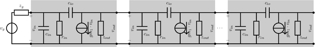
In general, multi-stage (opamp-like) amplifiers are used to circumvent the limitations of simple (single transistor) amplifiers. These opamp-like amplifiers consist of various cascaded amplifier stages. Usually one stage is dedicated to process differential input voltage into a current, another stage takes care of a high voltage gain or a high (trans)resistance and yet another amplification stage creates a low output impedance. This much more complex structure typically results in high voltage gain with a higher-order transfer function: every stage adds at least 1 order to the overall transfer function of the amplifier.

Creating a dominant first-order of a multi-stage amplifier is nothing more or less than moving one of the corner frequencies to a sufficiently low frequency. This is usually accomplished by adding a large capacitance to a high-ohmic internal node. An example of its effect on the open loop gain $A (jω)$ is shown in figure 6.21. Here, the lowest pole (at $1 0^{4} rad ∕ s$ in the original openloop gain $A (jω)$ ) was shifted to $10 rad ∕ s$ .

By shifting the low frequency corner frequency, a dominant first-order characteristic is obtained, at the cost of gain. In the Bode plot for this example, for the original open loop gain (in red), at unity gain feedback ( $β = 1$ ):

the phase margin is about $- 8 0^{\circ}$
the gain margin is approximately -30 dB
both indicate an unstable system

For the modified, dominant first order, openloop transfer

the phase margin is roughly $8 5^{\circ}$
the gain margin is 30 dB
both indicate a stable system

[prev] [prev-tail] [front] [up]